CNN 日常总结
Init
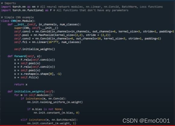
Xavier Init
可以使得CNN中layer与layer间的误差的方差保持稳定,既是让样本空间与类别空间的方差,差不多(趋于一样)。
pytorch 链接
kaiming初始化方法针对xavier初始化方法在relu这一类激活函数表现不佳而提出的改进
Pytorch example
Weight Decay
用于penalize complex model training. 一般用0.01(from fast.ai)
- 当parameters 有正有负时,直接传统的用“减”作为惩罚doesn’t work,因为对于负数的parameter来说,无法确定这是惩罚。 所以当parameters有正负情况发生时,使用square来解决。
- 但是Square会让loss增大特别快且明显。loss过大,会让model发生parameters全为0的情况。
- 所以weight decay就是为了防止model死了,添加的一个factor。
Batch size
一般用64.
把batch size往大了调主要是为了加快训练速度。但不一定保证训练的结果好坏。
Convolution Layer
How can Conv layer and pooling layer increase receptive field
Dialated Conv
Deformable conv
weighted
Input frame filter
entropy filter
Entropy masking is a useful technique that can help data scientists segment portions of an image by complexity. The applications range from texture analysis, image filtering, and even text extraction (a feature that can lend itself well to Natural Language Processing).
https://www.cs.cmu.edu/afs/cs/project/jair/pub/volume11/fox99a-html/node12.html
配合Particle filter可以用于定位.
Linear regression
要基本满足的条件:
- The Quantitative Data Condition.
- The Straight Enough Condition (or “linearity”).
- The Outlier Condition.
- Independence of Errors
- Homoscedasticity
- Normality of Error Distribution
1: 是数字data
2:确保数据是fit a line的,是linear的
3: outlier对regression 影响极大,最好run一遍带outlier的,另一遍不带outlier的
4:linear regression的error可以是random分布的,也可以是有特殊pattern的。error服从mean=0的正态分布
5: With homoscedasticity, you basically want your points to look like a tube instead of a cone.Error不会越来越大(小)
6:At any point in your x-values, the data points should be normally distributed around the regression line.
Independent Error
constant variance assumption(Variance of error is constant)
the average squared deviation of each error from the true regression model should be the same for every observation
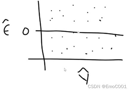
If above assumption is correct
then a plot of Error versus y or x should be random scatter, and the spread of residuals should have a constant thickness from left to right along the x-axis of plot. (errors are uncorrelated)
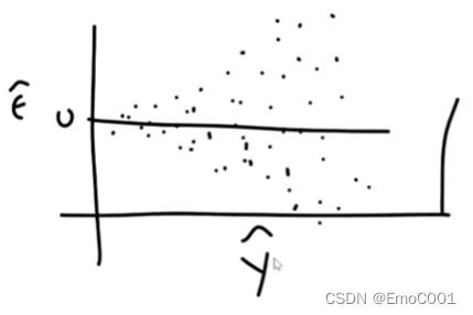
If above assumption is violated
then a plot of Error versus y or x will have a systematic, varying spread of residuals.
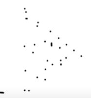
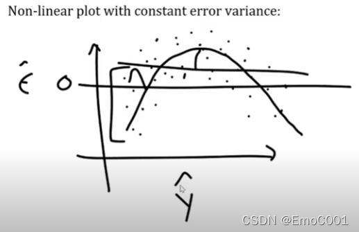
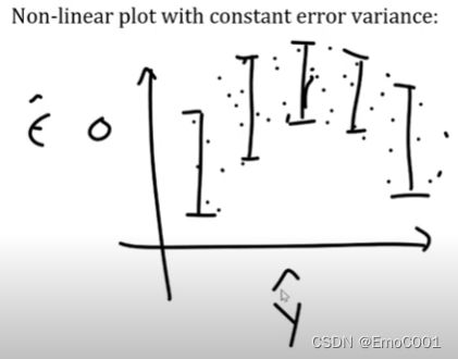
Constant error variance but non-linear plot
虽然图一的Error不是传统的随X轴均匀分布,但是如果把图一换成图二考虑,那么,Error是均匀的分布。
mean zero assumption
标准化,与PCA预处理操作类似
Normal Error distribution
Gradient Vanish

如何防止让多个gradients相乘结果接近0:
The farther x needs to move away from 0, the harder it is to produce a derivative below 1/n, thus, the easier it is to prevent the multiplication from vanishing.
当”X>1”的数量 == “X<1”的数量,gradient = 1
Extrs knowledges:
- Change y sign, get symmetry about x
- Change x sign, get symmetry about y
backpropagation 是关于loss function 的 derivation,为何与activatetion func 有联系
根据chain rule of partial derivatives:
loss func的derivation = a product of gradients of all the activation functions of the nodes with respect to their weights.
因此对nodes的weight 更新,完全取决于 gradients of the activation functions.
sigmoid
partial derivative of the sigmoid function reaches a maximum value of 0.25
Tanh
通常比Sigmoid好
Limitations of Sigmoid and Tanh Activation Functions
-
both the sigmoid and tanh functions is that they saturate. This means that large values snap to 1.0 and small values snap to -1 or 0 for tanh and sigmoid respectively。所以一个好的activate function不应该接受saturate的情况。
-
the functions are only really sensitive to changes around their mid-point of their input, such as 0.5 for sigmoid and 0.0 for tanh.
-
nonlinear 的计算对GPU不友好
-
nonlinear 的会使得用来update netwrok 的error减少,从而发生著名的“gradient vanish”事件
RELU: Sigmoid 与 Tanh的救世主
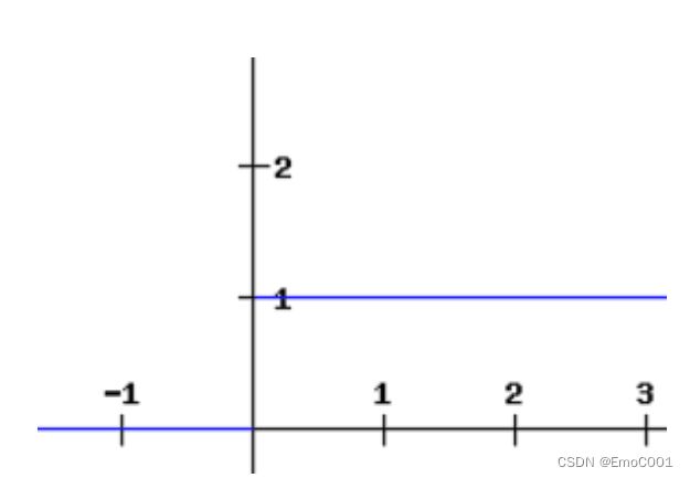
The derivative of a ReLU function is defined as 1 for inputs that are greater than zero and 0 for inputs that are negative.
But, RELU 的 dereivation 还是会让gradient 为 0 的情况。 因此,RELU的救世主就是LEAKY RELU
Upstream gradient
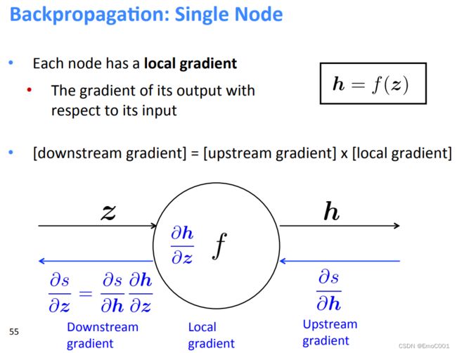
多个 inputs --> 多个 local gradients
stochastic gradient
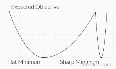
容易divergence. 由于Stogastic gradient 属于Small batch的方法,但是Large batch的方法通常比Small batch的方法更不容易stichastic. Small batch 会让search 的那个过程中错过optimal point,特别是 急转直下的那种,更容易进到flat minimum。如图:
logistic regression
与Feature关系很大,但改变trained model的Weight,对其结果不会有任何影响。
Layers
Dropout Layer
the outputs are scaled by a factor of $ \frac{1}{1-p}$ during training.
P: probability of an element to be zeroed
Fully connect Layer
When the model has an excessive number of parameters it becomes prone to overfitting.
以上问题均可以通过减少Layers 或者 neurons 改善overfitting
hyperparameters
- 当参数排列组合小时,使用grid search。
- 当参数排列组合大时,使用random search。
- 在选择一些数值上,使用log scale, 可以帮我们更快锁定optimal的区域,从而在那个区域附近进而摸索最优的参数。
Symmetry network (model compression)
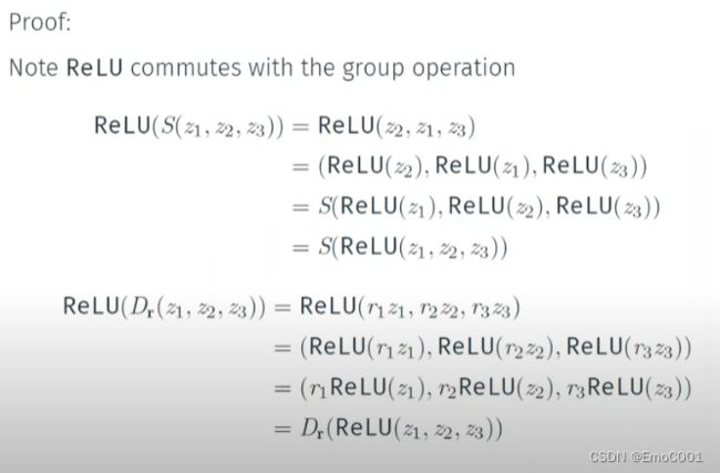
f ( g ( x ) ) = g ( f ( x ) ) f(g(x)) = g(f(x)) f(g(x))=g(f(x))
与 jesen’s inequlity 做区别: f ( ∑ p i x i ) ≤ ∑ p i f ( x i ) f(\sum p_i x_i) \leq \sum p_i f(x_i) f(∑pixi)≤∑pif(xi)
好处:
- 因为有些结构可以通过symmetry 的性质重复使用,因此,symmetry network 可以作为一个network compression的trick,从而减少parameters的数量。
- 例如: r e d u c e ( 1 , 8 , 16 , 8 , 1 ) = = ( 1 , 2 , 3 , 4 , 1 ) reduce(1,8,16,8,1)==(1,2,3,4,1) reduce(1,8,16,8,1)==(1,2,3,4,1)
TODO:
https://towardsdatascience.com/neural-network-breaking-the-symmetry-e04f963395dd
https://www.youtube.com/watch?v=8s0Ka6Y_kIM
Full batch, mini-batch, and online learning
The amount of data included in each sub-epoch weight change is known as the batch size. For example, with a training dataset of 1000 samples, a full batch size would be 1000, a mini-batch size would be 500 or 200 or 100, and an online batch size would be just 1.
在mini-batch里的gradient只能算作是approximate的
而 one batch 的 gradient,即确定的gradient(每个sample的gradient想加)
mini-batch的好处:
This reduces the risk of getting stuck at a local minimum, since different batches will be considered at each iteration, granting a robust convergence.
Although we don’t need to store the errors for the whole dataset in the memory, we still need to accumulate the sample errors to update the gradient after all mini-batches are evaluated.
Per-parameter adaptive learning rate methods
All previous approaches we’ve discussed so far manipulated the learning rate globally and equally for all parameters. Tuning the learning rates is an expensive process, so much work has gone into devising methods that can adaptively tune the learning rates, and even do so per parameter.
例子:
- Adagrad is an adaptive learning rate method
- RMSprop is a very effective, but currently unpublished adaptive learning rate method
- Adam. Adam is a recently proposed update that looks a bit like RMSProp with momentum
