Linear Regression Practice

import numpy as np
import pandas as pd
import matplotlib.pyplot as plt

Import other modules

from sklearn import linear_model
from sklearn.metrics import mean_squared_error
from sklearn.metrics import r2_score

Create function to obtain the train and test data

def getData(ticker, indx):
    # Construct the name of the files containing the ticker and the "index"
    ticker_file = "./data/assignment_1/{t}.csv".format(t=ticker)
    indx_file   = "./data/assignment_1/{t}.csv".format(t=indx)
    
    # Create the function body according to the spec
    ticker_data = pd.read_csv(ticker_file, usecols = [0,4], header = 0, names = ['Dates', 'Dependent'], index_col = 'Dates')
    indx_data = pd.read_csv(indx_file, usecols = [0,4], header = 0, names = ['Dates', 'Independent'], index_col = 'Dates')
    data = pd.merge(ticker_data, indx_data, on = 'Dates')

    # Change the return statement as appropriate
    return data

# Ticker: BA (Boeing), Index: SPY (the ETF for the S&P 500)
df = getData("BA", "SPY")

X = df.loc[:, ["Independent"] ]
y = df.loc[:, ["Dependent"] ]

df = getData("FB", "SPY")

X_FB = df.loc[:, ["Independent"] ]
y_FB = df.loc[:, ["Dependent"] ]

Create function to split the full data into train and test data

def split(X, y, seed=42):
    # Create the function body according to the spec
    X_train,  X_test = X.loc["2018-01-01":"2018-06-30"] , X.loc["2018-07-01":"2018-07-31"]
    y_train,  y_test = y.loc["2018-01-01":"2018-06-30"] , y.loc["2018-07-01":"2018-07-31"]
    
    # Change the return statement as appropriate
    return X_train, X_test, y_train, y_test
   

# Split the data into a training and a test set
X_train, X_test, y_train, y_test = split(X, y)
X_FB_train, X_FB_test, y_FB_train, y_FB_test = split(X_FB, y_FB)

Create a function to perform any other preparation of the data needed

Here, we need to turn the price data into price data. Remember to remove the first line of NA.

def prepareData( dfList ):
    # Create the function body according to the spec
    finalList = [0] * len(dfList)
    a = [0] * len(dfList)
    for i in range(len(dfList)) :
        finalList[i] = dfList[i].pct_change()
        a[i] = finalList[i].index[0]
        finalList[i] = finalList[i].drop([a[i]]) 
    result = tuple(finalList)
   # Change the return statement as appropriate
    return result

Transform the raw data, if needed

X_train, X_test, y_train, y_test = prepareData( [ X_train, X_test, y_train, y_test ] )

X_FB_train, X_FB_test, y_FB_train, y_FB_test = prepareData([X_FB_train, X_FB_test, y_FB_train, y_FB_test])

Create function to convert the DataFrames to ndarrays

def pd2ndarray( dfList ):
    # Create the function body according to the spec
    data_arrays = [0]*len(dfList)
    for i in range(len(dfList)) :
        data_arrays[i] = np.array(dfList[i])
    
    result = tuple(data_arrays)
    # Change the return statement as appropriate
    return result
   

X_train, X_test, y_train, y_test = pd2ndarray( [X_train, X_test, y_train, y_test] )
X_FB_train, X_FB_test, y_FB_train, y_FB_test = pd2ndarray([X_FB_train, X_FB_test, y_FB_train, y_FB_test])

Create function to return the sklearn model you need

def createModel():
    # Create the function body according to the spec
    regr = linear_model.LinearRegression()
    
    # Change the return statement as appropriate
    return regr

# Create linear regression object
model = createModel()

# Train the model using the training sets
_ = model.fit(X_train, y_train)

# The coefficients
print('Coefficients: \n', model.intercept_, model.coef_)

Coefficients: 
 [0.0010151] [[1.35452489]]

# Create linear regression object
model_FB = createModel()

# Train the model using the training sets
_ = model_FB.fit(X_FB_train, y_FB_train)

# The coefficients
print('Coefficients: \n', model_FB.intercept_, model_FB.coef_)

Coefficients: 
 [0.0005995] [[1.20737853]]

Create function to compute a Root Mean Squared Error

def computeRMSE( target, predicted ):
    # Create the function body according to the spec
    rmse = np.sqrt(mean_squared_error(target, predicted))
        
    # Change the return statement as appropriate
    return rmse

Evaluate in and out of sample Root Mean Squared Error

# Predictions:
# predict out of sample: 
y_pred_test = model.predict( X_test )

# predict in sample: 
y_pred_train = model.predict( X_train )

# Compute the in-sample fit
rmse_insample = computeRMSE( y_train, y_pred_train )
print("RMSE (train): {r:2.3f}".format(r=rmse_insample))

# Compute the out of sample fit
rmse_outOfsample = computeRMSE( y_test, y_pred_test)
print("RMSE (test): {r:2.3f}".format(r=rmse_outOfsample))

RMSE (train): 0.014
RMSE (test): 0.011

The RMSE is small, but it does not mean the model is perfect. Let’s see the R square and we will find that the R Square for both models of BA and FB is very small.

R2_BA_test = r2_score(y_test, y_pred_test )
R2_BA_train = r2_score(y_train, y_pred_train)
R2_BA_train, R2_BA_test

(0.48968697821649876, 0.3126888575743322)

# Predictions:
# predict out of sample: 
y_FB_pred_test = model_FB.predict( X_FB_test )

# predict in sample: 
y_FB_pred_train = model_FB.predict( X_FB_train )

# Compute the in-sample fit
rmse_insample = computeRMSE( y_FB_train, y_FB_pred_train )
print("RMSE (train): {r:2.3f}".format(r=rmse_insample))

# Compute the out of sample fit
rmse_outOfsample = computeRMSE( y_FB_test, y_FB_pred_test)
print("RMSE (test): {r:2.3f}".format(r=rmse_outOfsample))

RMSE (train): 0.016
RMSE (test): 0.043

R2_FB_test = r2_score(y_FB_test, y_FB_pred_test )
R2_FB_train = r2_score(y_FB_train, y_FB_pred_train)
R2_FB_train, R2_FB_test

(0.3894497290195409, 0.06288710943458953)

Q1 : Thoughts/theories on the insample vs out of sample performance

It seems that the performace of out of sample and the insample is very good(since the RSME is very small). But it does not mean that it’s a good model or the model provide a very nice prediction. One of the reasons is that the absolute value of the returns is very small, so the RMSE is definitely not big. When we check the R2 out of sample of each model, we will find that the R2 is very small. Another important reason is that we need to change the training set and test set to evaluate the performance(We will discusss that in the extra credit part). Another reason is that the test set is very small, we need to enlarge the test set to see what happens. In order to see that, we have to explore more on the test set. What will happen when the test set is from 2018-07-01 to 2018-08-31 or even later? Lets see the code below

x_test_long = [0]*6
y_test_long = [0]*6
        
x_test_long[0], y_test_long[0] = X.loc["2018-07-01":"2018-07-31"], y.loc["2018-07-01":"2018-07-31"]
x_test_long[1], y_test_long[1] = X.loc["2018-07-01":"2018-08-31"], y.loc["2018-07-01":"2018-08-31"]
x_test_long[2], y_test_long[2] = X.loc["2018-07-01":"2018-09-28"], y.loc["2018-07-01":"2018-09-28"]
x_test_long[3], y_test_long[3] = X.loc["2018-07-01":"2018-10-31"], y.loc["2018-07-01":"2018-10-31"]
x_test_long[4], y_test_long[4] = X.loc["2018-07-01":"2018-11-30"], y.loc["2018-07-01":"2018-11-30"]
x_test_long[5], y_test_long[5] = X.loc["2018-07-01":"2018-12-31"], y.loc["2018-07-01":"2018-12-31"]

x_test_long = list(prepareData(x_test_long))
y_test_long = list(prepareData(y_test_long))
    
x_test_long = list(pd2ndarray(x_test_long))
y_test_long = list(pd2ndarray(y_test_long))

rmse_outOfsample_long = [0]*6
y_pred_test_long = [0]*6

for i in range(6):
    y_pred_test_long[i] = model.predict( x_test_long[i] )
    rmse_outOfsample_long[i] = computeRMSE(y_test_long[i], y_pred_test_long[i] )


dataList = ['July', 'August', 'September', 'Octobor', 'November', 'December']
long_test_sample_error = pd.DataFrame(rmse_outOfsample_long, columns = ['Out of sample RMSE'] , index = dataList)
long_test_sample_error

	Out of sample RMSE
July	0.010557
August	0.010723
September	0.010945
Octobor	0.013606
November	0.013646
December	0.013647

long_test_sample_error.plot()

Then we can find that the performance of the model behaves not well after september and the change is sharply. The reason is that the predictors need more information.(There maybe new trends in the market)

r2_long = [0]*6

for i in range(6):
    r2_long[i] = r2_score(y_test_long[i], y_pred_test_long[i] )


dataList = ['July', 'August', 'September', 'Octobor', 'November', 'December']
r2_long_sample = pd.DataFrame(r2_long, columns = ['Out of sample R2'] , index = dataList)
r2_long_sample

	Out of sample R2
July	0.312689
August	0.325917
September	0.251906
Octobor	0.312820
November	0.385558
December	0.514831

Q2 : Comparison with FB

Plot the predicted(red) and true(black) of BA and FB

fig = plt.figure()
ax = fig.add_subplot(121)
_ = ax.scatter(X_train, y_train, color = 'black', label = "test")
_ = ax.scatter(X_train, y_pred_train, color = 'red', label = "predicted")
_ = ax.set_xlabel("SPY return")
_ = ax.set_ylabel("BA return")
_ = ax.legend()
ax = fig.add_subplot(122)
_ = ax.scatter(X_test, y_test, color = 'black', label = "test")
_ = ax.scatter(X_test, y_pred_test, color = 'red', label = "predicted")
_ = ax.set_xlabel("SPY return")
_ = ax.set_ylabel("BA return")
_ = ax.legend()

In BA case, The true value is evenly distributed on both sides of the fitted line both in train set and in test set. So the root mean squared loss is small.

fig = plt.figure()
ax = fig.add_subplot(121)
_ = ax.scatter(X_FB_train, y_FB_train, color = 'black', label = "test")
_ = ax.scatter(X_FB_train, y_FB_pred_train, color = 'red', label = "predicted")
_ = ax.set_xlabel("SPY return")
_ = ax.set_ylabel("FB return")
_ = ax.legend()
ax = fig.add_subplot(122)
_ = ax.scatter(X_FB_test, y_FB_test, color = 'black', label = "test")
_ = ax.scatter(X_FB_test, y_FB_pred_test, color = 'red', label = "predicted")
_ = ax.set_xlabel("SPY return")
_ = ax.set_ylabel("FB return")
_ = ax.legend()

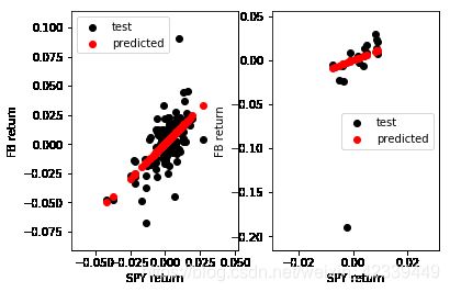
In FB case, there are some outliers in the dataset, so that the result seems not as good as BA case. But if we delete the outliers from the test set, we will find that the performance of the model in the FB case will be much better in FB case.

Now, lets go back to the start point, to see how does the original data behave :

data_BAFB = pd.merge(df, y , on = 'Dates')
data_BAFB.columns = ['FB', 'SPY', 'BA']
data_return = data_BAFB.pct_change()
data_return.drop("2018-01-02")
data_return.plot()

data_return.hist()

data_return.describe()

	FB	SPY	BA
count	250.000000	250.000000	250.000000
mean	-0.001003	-0.000232	0.000528
std	0.023949	0.010804	0.019853
min	-0.189609	-0.041823	-0.065911
25%	-0.010744	-0.005062	-0.010187
50%	0.000374	0.000268	-0.000817
75%	0.011473	0.005442	0.012516
max	0.090613	0.050525	0.067208

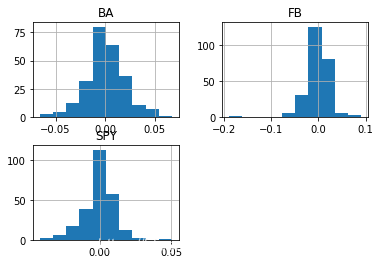
From the two graphs above, we can find that BA’s distribution is similar to SPY. However, FB has more outliers. From the description table, we can see that all of the three timeseries’ mean is approximately 0. FB has a bigger variance. The range of FB is much bigger than the other two. So the reason why that FB behaves not well in the model is that it contains some outliers.

Q3 : What will happen if we use other timeseries as estimators?

Part One : Loading all the data in the files

X_GS = pd.read_csv("./data/assignment_1/GS.csv", usecols = [0,4], header = 0, names = ['Dates', 'GS'], index_col = 'Dates')
X_MRK = pd.read_csv("./data/assignment_1/MRK.csv", usecols = [0,4], header = 0, names = ['Dates', 'MRK'], index_col = 'Dates')
X_PFE = pd.read_csv("./data/assignment_1/PFE.csv", usecols = [0,4], header = 0, names = ['Dates', 'PFE'], index_col = 'Dates')
X_QQQ = pd.read_csv("./data/assignment_1/QQQ.csv", usecols = [0,4], header = 0, names = ['Dates', 'QQQ'], index_col = 'Dates')
X_VZ = pd.read_csv("./data/assignment_1/VZ.csv", usecols = [0,4], header = 0, names = ['Dates', 'VZ'], index_col = 'Dates')
X_WMT = pd.read_csv("./data/assignment_1/WMT.csv", usecols = [0,4], header = 0, names = ['Dates', 'WMT'], index_col = 'Dates')
X_XLK = pd.read_csv("./data/assignment_1/GS.csv", usecols = [0,4], header = 0, names = ['Dates', 'XLK'], index_col = 'Dates')
estimator_list = [X, X_GS, X_MRK, X_PFE, X_QQQ, X_VZ, X_WMT, X_XLK]

Part Two : Fit in the model with each estimator

def Fit_in_Model(X, Y) :
    ###Prepare data
    X_train, X_test, y_train, y_test = split(X, Y)
    X_train, X_test, y_train, y_test = prepareData( [ X_train, X_test, y_train, y_test ] )
    X_train, X_test, y_train, y_test = pd2ndarray( [X_train, X_test, y_train, y_test] )
    
    ###Fit the model
    model = createModel()
    _ = model.fit(X_train, y_train)
    y_pred_test = model.predict( X_test )
    y_pred_train = model.predict( X_train )
    rmse_insample = computeRMSE( y_train, y_pred_train )
    rmse_outOfsample = computeRMSE( y_test, y_pred_test)
    
    return y_pred_test, y_pred_train, rmse_insample, rmse_outOfsample
    

y_pred_BA_test = [0]*8
y_pred_BA_train = [0]*8
rmse_BA_insample = [0]*8
rmse_BA_outOfsample = [0]*8
r2_score_BA = [0]*8
for i in range(len(estimator_list)) :
    y_pred_BA_test[i], y_pred_BA_train[i], rmse_BA_insample[i], rmse_BA_outOfsample[i]= Fit_in_Model(y, estimator_list[i])

nameList = ['SPY', 'GS', 'MRK', 'PFE', 'QQQ', 'VZ', 'WMT', 'XLK']
errorList = [rmse_BA_insample, rmse_BA_outOfsample]
error_compare = pd.DataFrame(errorList, columns = nameList, index = ['rmse_BA_insample', 'rmse_BA_outOfsanple'])
error_compare

	SPY	GS	MRK	PFE	QQQ	VZ	WMT	XLK
rmse_BA_insample	0.007414	0.012651	0.013267	0.010908	0.010182	0.013003	0.015043	0.012651
rmse_BA_outOfsanple	0.004783	0.009510	0.009863	0.009421	0.008967	0.009858	0.006838	0.009510

Part Three : Compare the results

error_compare.T.plot.bar()

y_pred_FB_test = [0]*8
y_pred_FB_train = [0]*8
rmse_FB_insample = [0]*8
rmse_FB_outOfsample = [0]*8
for i in range(len(estimator_list)) :
    y_pred_FB_test[i], y_pred_FB_train[i], rmse_FB_insample[i], rmse_FB_outOfsample[i] = Fit_in_Model(y_FB, estimator_list[i])
errorList_FB = [rmse_FB_insample, rmse_FB_outOfsample]
error_compare_FB = pd.DataFrame(errorList_FB, columns = nameList, index = ['rmse_FB_insample', 'rmse_FB_outOfsanple'])

error_total = pd.concat([error_compare, error_compare_FB])
error_total.T.plot.bar()

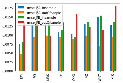
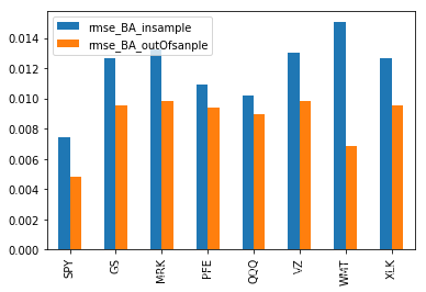
Through the experiment above, we can easily find that in one estimator case:
for BA, SPY is the best estimator.
for FB, MRK is the best estimator.

Part Four : What will happen when it comes to Multiple Linear Regression?

## Join together
data_total = pd.concat([y]+estimator_list, axis = 1)
data_total = data_total.pct_change()
data_total = data_total.drop("2018-01-02")
data_total.rename(columns={ data_total.columns[1]: "SPY" }, inplace=True)

## Looking for correlations
import seaborn as sns
corr_matrix = data_total.corr()
sns.heatmap(corr_matrix)
corr_matrix

	Dependent	SPY	GS	MRK	PFE	QQQ	VZ	WMT	XLK
Dependent	1.000000	0.709471	0.554255	0.332268	0.409477	0.644716	0.213725	0.396931	0.554255
SPY	0.709471	1.000000	0.770636	0.582286	0.681485	0.947075	0.376749	0.494996	0.770636
GS	0.554255	0.770636	1.000000	0.436829	0.461078	0.704788	0.272062	0.360350	1.000000
MRK	0.332268	0.582286	0.436829	1.000000	0.634451	0.479143	0.402445	0.424872	0.436829
PFE	0.409477	0.681485	0.461078	0.634451	1.000000	0.582679	0.397530	0.425178	0.461078
QQQ	0.644716	0.947075	0.704788	0.479143	0.582679	1.000000	0.230613	0.383508	0.704788
VZ	0.213725	0.376749	0.272062	0.402445	0.397530	0.230613	1.000000	0.378218	0.272062
WMT	0.396931	0.494996	0.360350	0.424872	0.425178	0.383508	0.378218	1.000000	0.360350
XLK	0.554255	0.770636	1.000000	0.436829	0.461078	0.704788	0.272062	0.360350	1.000000

From the chart above, we can find that SPY and QQQ has the biggest correlation with BA. The result is correspond to the result of one estimator. Now, lets try multiple linear regression.

X_data = pd.concat(estimator_list, axis = 1)
X_data.rename(columns={ X_data.columns[0]: "SPY" }, inplace=True)

from sklearn.linear_model import Lasso
from sklearn.linear_model import Ridge
from sklearn.linear_model import ElasticNet

def data_pipeline(X, Y) :
    X_train, X_test, y_train, y_test = split(X, Y)
    X_train, X_test, y_train, y_test = prepareData( [ X_train, X_test, y_train, y_test ] )
    X_train, X_test, y_train, y_test = pd2ndarray( [X_train, X_test, y_train, y_test] )
    return X_train, X_test, y_train, y_test

def MLR_Models(X, Y) :
    ###Prepare data
    X_train_M, X_test_M, y_train_M, y_test_M = data_pipeline(X, Y)
    
    ###Fit the model
    model1 = createModel()
    model2 = linear_model.Lasso(alpha = 0.5)
    model3 = linear_model.Ridge(alpha = 0.5)
    model4 = linear_model.ElasticNet(alpha = 0.5, l1_ratio = 0.5)
    
    models = [model1, model2, model3, model4]
    y_pred_test = [0]*4
    y_pred_train = [0]*4
    rmse_insample = [0]*4
    rmse_outOfsample = [0]*4
    
    for i in range(4) :
        y_pred_test[i] = models[i].fit(X_train_M, y_train_M).predict( X_test_M )
        y_pred_train[i] = models[i].fit(X_train_M, y_train_M).predict( X_train_M )
        rmse_insample[i] = computeRMSE( y_train_M, y_pred_train[i])
        rmse_outOfsample[i] = computeRMSE( y_test_M, y_pred_test[i])
        
    return y_pred_test, y_pred_train, rmse_insample, rmse_outOfsample

y_pred_BA_test, y_pred_BA_train, rmse_BA_insample, rmse_BA_outOfsample = MLR_Models(X_data, y)
y_pred_FB_test, y_pred_FB_train, rmse_FB_insample, rmse_FB_outOfsample = MLR_Models(X_data, y_FB)
method_name = ['Linear Regression', 'Lasso Regression', 'Ridge Regression', 'ElasticNet Regression']
error_M_BAFB = [rmse_BA_insample, rmse_BA_outOfsample, rmse_FB_insample, rmse_FB_outOfsample,]
error_M_BAFB = pd.DataFrame(error_M_BAFB, columns = method_name, index = ['rmse_BA_insample', 'rmse_BA_outOFsample', 'rmse_FB_insample', 'rmse_FB_outOFsample'])
error_M_BAFB

	Linear Regression	Lasso Regression	Ridge Regression	ElasticNet Regression
rmse_BA_insample	0.013501	0.020090	0.018754	0.020090
rmse_BA_outOFsample	0.010311	0.012863	0.012260	0.012863
rmse_FB_insample	0.014444	0.020081	0.019075	0.020081
rmse_FB_outOFsample	0.038764	0.044812	0.044503	0.044812

It seems that the performance of the Multiple Linear Regression is much worse than the one estimator case. But remember, there are still parameters such as numbers of the estimators, Alpha, l1_ratio can still be changed in order to improve the performance. So, we need to use method such as Grid Search to do hyperparameter tuning. But I don’t want to dive deep here, for I guess the result of MLR won’t be very good because of the high correlations between the features. What I want to try is to add a new dimonsion $x^2$

Part Five : What will happen if we add a new dimonsion $x^2$ ?

Lets first look at the scatter graph of the X_train and y_train. The relationship between X and Y is likely to be a quadratic function.

fig = plt.figure()
ax = fig.add_subplot(121)
_ = ax.scatter(X_train, y_train, color = 'black', label = "BA")
_ = ax.set_xlabel("Return of SPY")
_ = ax.set_ylabel("Return of BA")
_ = ax.legend()
ax = fig.add_subplot(122)
_ = ax.scatter(X_FB_train, y_FB_train, color = 'red', label = "FB")
_ = ax.set_xlabel("Return of SPY")
_ = ax.set_ylabel("Return of FB")
_ = ax.legend()

def Quadratic_transfor(X) :
    X_2 = np.concatenate([X,X**2], axis = 1)
    return X_2

X_train_2 = Quadratic_transfor(X_train)
X_test_2 = Quadratic_transfor(X_test)
X_FB_train_2 = Quadratic_transfor(X_FB_train)
X_FB_test_2 = Quadratic_transfor(X_FB_test)

def Fit_Model(X_train, X_test, y_train, y_test) :
    
    ###Fit the model
    model = createModel()
    _ = model.fit(X_train, y_train)
    y_pred_test = model.predict( X_test )
    y_pred_train = model.predict( X_train )
    rmse_insample = computeRMSE( y_train, y_pred_train )
    rmse_outOfsample = computeRMSE( y_test, y_pred_test)
    
    return rmse_insample, rmse_outOfsample, y_pred_test, y_pred_train

BA_QU_rmse_insample, BA_QU_rmse_outOfsample, BA_pred_test_QU, BA_pred_train_QU = Fit_Model(X_train_2, X_test_2, y_train, y_test )
FB_QU_rmse_insample, FB_QU_rmse_outOfsample, FB_pred_test_QU, FB_pred_train_QU = Fit_Model(X_FB_train_2, X_FB_test_2, y_FB_train, y_FB_test )

error_QU = {'BA':[BA_QU_rmse_insample, BA_QU_rmse_outOfsample], 'FB': [FB_QU_rmse_insample, FB_QU_rmse_outOfsample]}
error_QU_df = pd.DataFrame(error_QU, index = ['Insample Error', 'Outofsample Error'])

fig = plt.figure()
ax = fig.add_subplot(221)
_ = ax.scatter(X_train, y_train, color = 'black', label = "test")
_ = ax.scatter(X_train, BA_pred_train_QU, color = 'red', label = "predicted")
_ = ax.set_xlabel("SPY return")
_ = ax.set_ylabel("BA return")
_ = ax.legend()
ax = fig.add_subplot(222)
_ = ax.scatter(X_test, y_test, color = 'black', label = "test")
_ = ax.scatter(X_test, BA_pred_test_QU, color = 'red', label = "predicted")
_ = ax.set_xlabel("SPY return")
_ = ax.set_ylabel("BA return")
_ = ax.legend()
ax = fig.add_subplot(223)
_ = ax.scatter(X_FB_train, y_FB_train, color = 'black', label = "test")
_ = ax.scatter(X_FB_train, FB_pred_train_QU, color = 'red', label = "predicted")
_ = ax.set_xlabel("SPY return")
_ = ax.set_ylabel("FB return")
_ = ax.legend()
ax = fig.add_subplot(224)
_ = ax.scatter(X_FB_test, y_FB_test, color = 'black', label = "test")
_ = ax.scatter(X_FB_test, FB_pred_test_QU, color = 'red', label = "predicted")
_ = ax.set_xlabel("SPY return")
_ = ax.set_ylabel("FB return")
_ = ax.legend()

R2_QU_BA = r2_score(y_test, BA_pred_test_QU )
R2_QU_FB = r2_score(y_FB_test, FB_pred_test_QU)
R2_QU_BA, R2_QU_FB

(0.3139138387590181, 0.05607453030855791)

After trying $X^2$, we find that the performance of this model is not better than the previous one not only on the metric of RMSE but also on the R square.

Q4 : What will happen when we change the data range of our training data ?

X_training_df_original, y_training_df_original = X.loc['2018-01-02':'2018-06-30'], y.loc['2018-01-02':'2018-06-30']
X_training_df_original, y_training_df_original = X_training_df_original.pct_change(), y_training_df_original.pct_change()

X_training_df_original, y_training_df_original = X_training_df_original.drop("2018-01-02"), y_training_df_original.drop("2018-01-02")
X_training_array, y_training_array = pd2ndarray([X_training_df_original, y_training_df_original])

X_training_array_list = [0]*len(X_training_array)
y_training_array_list = [0]*len(y_training_array)
for i in range(len(X_training_array)) :
    X_training_array_list[i] = X_training_array[i:]
    y_training_array_list[i] = y_training_array[i:]

def Fit_Model2(X_train, X_test, y_train, y_test) :
    
    ###Fit the model
    model = createModel()
    _ = model.fit(X_train, y_train)
    y_pred_test = model.predict( X_test )
    y_pred_train = model.predict( X_train )
    rmse_insample = computeRMSE( y_train, y_pred_train )
    rmse_outOfsample = computeRMSE( y_test, y_pred_test)
    
    return rmse_insample, rmse_outOfsample

rmse_t_insample = [0]*len(X_training_array_list)
rmse_t_outOfsample = [0]*len(X_training_array_list)
for i in range(len(X_training_array_list)) :
    rmse_t_insample[i], rmse_t_outOfsample[i] = Fit_Model2(X_training_array_list[i], X_test, y_training_array_list[i], y_test)

insample_reverse = rmse_t_insample[::-1]
outsample_reverse = rmse_t_outOfsample[::-1]

Train_change_insample = pd.DataFrame(insample_reverse, columns = ['insample'])
Train_change_insample.plot().set_xlabel('Numbers of data in training set')

Train_change_outOfsample = pd.DataFrame(outsample_reverse, columns = ['out of sample'])
Train_change_outOfsample.plot().set_xlabel('Numbers of data in training set')

We can conclude that as the number of data in training set increase, the RMSF of the test set will decrease.

Q5 : Show a scatter plot of error versus distance from date of last training point

errors_BA = y_pred_test - y_test
errors_BA_abs = abs(y_pred_test - y_test)
num_days = np.arange(1, len(errors_BA)+1)

fig = plt.figure()
ax = fig.add_subplot(121)
_ = ax.scatter(num_days, errors_BA, color = 'black', label = "BA errors")
_ = ax.set_xlabel("Days from date of last training point")
_ = ax.set_ylabel("BA errors")
_ = ax.legend()
ax = fig.add_subplot(122)
_ = ax.scatter(num_days, errors_BA_abs, color = 'red', label = "BA absolute errors")
_ = ax.set_xlabel("Days from date of last training point")
_ = ax.set_ylabel("BA absolute errors")
_ = ax.legend()

errors_BA_long = y_pred_test_long[5] - y_test_long[5]
errors_BA_abs_long = abs(y_pred_test_long[5] - y_test_long[5])
num_days_long = np.arange(1, len(errors_BA_long)+1)

fig = plt.figure()
ax = fig.add_subplot(121)
_ = ax.scatter(num_days_long, errors_BA_long, color = 'black', label = "BA errors")
_ = ax.set_xlabel("Days from date of last training point")
_ = ax.set_ylabel("BA errors")
_ = ax.legend()
ax = fig.add_subplot(122)
_ = ax.scatter(num_days_long, errors_BA_abs_long, color = 'red', label = "BA absolute errors")
_ = ax.set_xlabel("Days from date of last training point")
_ = ax.set_ylabel("BA absolute errors")
_ = ax.legend()

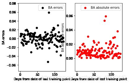
So, from the graph above, we can find that the absolute errors increase as it getting far away from the last training point in the first month. But if we enlarge our test set, we will find that the absolute errors stays nearly the same! But there will be more points that show great errors between the test and predicted set.

Q6 : Considerations of shuffling data when we are dealing with timeseries

Timeseries data often contains autocorrelation information. Suppose that we have a time series data :
$$TimeSeries=\left\{X_1,X_2,X_3,X_4,X_5,...,X_{98},X_{99},X_{100}\right\}{F}_i=\left\{X_1,X_2,X_3,...,X_i\right\}$$
$X_i$ is the ith element in the time series. $F_i$ is the information set of the ith element.

If we shuffle the dataset and get the training set and test set, we will find that the traing set contains part of the information in the test set.
$$Traingset=\left\{X_1,X_2,X_4,X_6,...,X_{99},X_{100}\right\}Testset=\left\{X_3,X_5,...,X_{98}\right\}$$
In another words, when we use the model to predict the future, the data we use has already contains the future information. The data in traing set has already contains the part of the trend information of $X_3,X_5,X_{98}$ It’s a kind of cheat.