强化学习算法实践（一）——策略梯度算法

文章目录

Reference
1. REINFORCE
- 1.1 Basic
- 1.2 Code
2. Improvement Tips
- 2.1 Assign Suitable Credit
- 2.2 Add a Baseline
- 2.3 Advantage Function
3. Actor-Critic(A2C)
- 3.1 Basic
- 3.2 Code

策略梯度是一种基于策略的算法，相比于DQN一类的基于价值的算法，它会直接显式的学习一个目标策略。梯度下降的基础知识可以参考之前的博客强化学习（六）策略梯度和《动手学强化学习》部分内容。

Reference

[1] 《动手学强化学习》 https://hrl.boyuai.com/
[2] David Silver: https://www.youtube.com/watch?v=KHZVXao4qXs&t=4609s

我们假设目标策略 $\pi_\theta(a|s)$ 是一种随机策略，并且处处可微， $\theta$ 为对应参数。可以通过神经网络或线性模型对目标策略进行建模。输入某个状态，输出动作的概率分布。
（1）目标函数
我们期望获得一个最优策略，能够最大化策略在环境中的期望回报。
$J(\theta)=E[V^{\pi_\theta}(s)]$

根据贝尔曼方程，我们可以用Q函数表示目标函数
$J(\theta)=\sum_{s \in S} d(s) \sum_{a \in A} \pi_\theta(a|s) Q^{\pi_\theta}(s,a)$

（2）梯度
我们希望通过梯度下降（上升）优化策略，策略梯度可以表示为
$\nabla \theta = \alpha \nabla J(\theta) \\ \nabla J(\theta) = \sum_{s \in S} d(s) \sum_{a \in A} \nabla \pi_\theta(a|s) Q^{\pi_\theta}(s,a)=E_{\pi_\theta}[Q^{\pi_\theta}(s,a) \nabla \log \pi_\theta(a|s)]$

因此我们可以将 $Q^{\pi_\theta}(s,a) \log \pi_\theta(a|s)$ 作为损失值反向传递优化模型。

1. REINFORCE

1.1 Basic

上文我们提到可以将 $Q^{\pi_\theta}(s,a) \log \pi_\theta(a|s)$ 作为损失值反向传递优化模型。我们在强化学习（五）价值函数拟合中学到可以通过MC或TD近似Q或V函数。REINFORCE算法就是采用MC方法，利用轨迹的累计回报预估Q函数，所以策略梯度改变成为：
$\nabla \theta = \alpha \nabla J(\theta) \\ \nabla J(\theta) =E_{\pi_\theta}[G_t \nabla \log \pi_\theta(a|s)]$

其中G_t是一条完整轨迹获得的累积奖励。REINFORCE是一种在线学习方法，采样到的轨迹数据只能使用一次。同时因为使用累计回报 $G_t$ 预测Q函数，所以算法的性能有一定程度的波动（高方差）。

1.2 Code

import gym
import torch
import torch.nn.functional as F
import numpy as np
import matplotlib.pyplot as plt
from tqdm import tqdm
import rl_utils

首先定义策略网络PolicyNet，输入是某个状态，输出则是该状态下的动作概率分布。

class PolicyNet(torch.nn.Module):
    def __init__(self, state_dim, hidden_dim, action_dim):
        super(PolicyNet, self).__init__()
        self.fc1 = torch.nn.Linear(state_dim, hidden_dim)
        self.fc2 = torch.nn.Linear(hidden_dim, action_dim)
        
    def forward(self, x):
        x = F.relu(self.fc1(x))
        return F.softmax(self.fc2(x), dim=1) # dim=1，对每行使用softmax

接着定义REINFORCE算法，take_action和update是算法最重要的两个部分。在take_action中通过由PolicyNet计算获得的动作概率分布和distribution.Categorical对离散动作采样。在update中，根据与环境交互记录的轨迹计算累积回报 $G_t$ ，并将损失函数设定为 $-G_t \nabla \log \pi_\theta(a|s)$ ，利用梯度下降优化模型。

class REINFORCE:
    def __init__(self, state_dim, hidden_dim, action_dim, 
                learning_rate, gamma, device):
        self.policy_net = PolicyNet(state_dim, hidden_dim, 
                                    action_dim).to(device)
        self.optimizer = torch.optim.Adam(self.policy_net.parameters(),
                                         lr=learning_rate)
        self.gamma = gamma
        self.device = device
    
    # 根据动作概率分布随机采样
    def take_action(self, state):
        state = torch.tensor([state], dtype=torch.float).to(self.device)
        probs = self.policy_net(state)
        
        action_dist = torch.distributions.Categorical(probs)
        action = action_dist.sample()
        return action.item()
    
    def update(self, transition_dict):
        reward_list = transition_dict['rewards']
        state_list = transition_dict['states']
        action_list = transition_dict['actions']
        
        G = 0
        self.optimizer.zero_grad()
        # 通过计算累积奖励G，获得梯度
        for i in reversed(range(len(reward_list))):
            reward = reward_list[i]
            state = torch.tensor([state_list[i]],
                                dtype=torch.float).to(self.device)
            action = torch.tensor([action_list[i]]).view(-1,1).to(self.device)
            
            log_prob = torch.log(self.policy_net(state).gather(1,action))
            G = self.gamma * G + reward
            
            loss = -log_prob * G # 梯度上升
            loss.backward()
        self.optimizer.step()

问题：如何计算 $\log \pi_\theta(a|s)$ ?怎么理解log_prob = torch.log(self.policy_net(state).gather(1,action))?

定义完策略后，我们可以在车杆环境上实验：

return_list = []
for i_episode in range(num_episodes):
    episode_return = 0
    transition_dict = {
        'states': [],
        'actions': [],
        'next_states': [],
        'rewards': [],
        'dones': []
    }
    state = env.reset()
    done = False
    while not done:
        action = agent.take_action(state)
        next_state, reward, done, _ = env.step(action)
        transition_dict['states'].append(state)
        transition_dict['actions'].append(action)
        transition_dict['next_states'].append(next_state)
        transition_dict['rewards'].append(reward)
        transition_dict['dones'].append(done)
        state = next_state
        episode_return += reward
    return_list.append(episode_return)
    # on-policy: learning from a trajectory
    agent.update(transition_dict)
    
    if (i_episode + 1) % 100 == 0:
        print(f'Episode: {i_episode + 1}, return={np.mean(return_list[-100:])}')

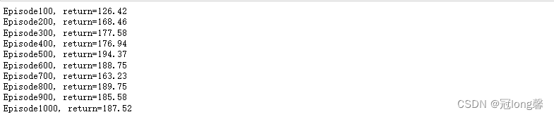
在1000次训练过程中我们发现，REINFORCE算法表现并不平稳，获得的return值时高时低。这是因为REINFORCE采用轨迹的累积回报预测Q函数具有较高的方差，因为采样轨迹差别过大而导致表现时好时坏。
训练完agent后，我们可以在实验环境中看看实际表现的效果如何

for i in range(5):
    episode_return = 0
    state = env.reset()
    done = False
    while not done:
        action = agent.take_action(state)
        next_state, reward, done, _ = env.step(action)
        env.render()
        state = next_state
        episode_return += reward
    print(episode_return)

2. Improvement Tips

正如上文所述，REINFORCE是一种具有无偏、高方差、低数据使用效率特点的On-Policy方法。我们需要设计一些技巧改进这样的方法。相关内容我在强化学习算法（五）——PPO中已经学习过了，此处尝试将他们串联起来。

2.1 Assign Suitable Credit

REINFORCE中的策略梯度为
$\nabla J(\theta)=-G_t \nabla \log \pi_\theta(a|s)$

其中 $\nabla \log \pi_\theta(a|s)$ 表示轨迹中每个状态动作对发生概率修正的方向（梯度方向）， $G_t$ 表示每个状态动作对发生概率修正的权重（大小与方向）。因此，在同一条轨迹中的所有状态动作对修正的权重相同。

很明显我们并不期望所有状态动作对的变化程度相同，所以我们需要修改G_t。我们使用状态动作对(s,a)发生后的累积奖励 $\sum_{t'=0}^T \gamma^{t'-t} R_{t'}$ 作为每个状态动作对的修正权重，从而保证了每个状态动作对修正权重的独特性。
$\nabla J(\theta)=- (\sum_{t'=0}^T \gamma^{t'-t} R_{t'}) \nabla \log \pi_\theta(a|s)$

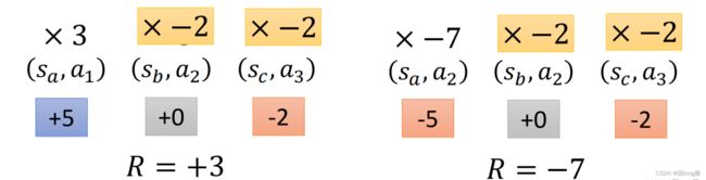
2.2 Add a Baseline

假设采样获得的所有状态动作对的累积奖励均大于0.在理想状态下，a, b, c三种状态动作对都被采样，状态动作的发生概率都获得了提高。但实际情况并不能保证采样到所有状态动作对，没被采样的状态动作对的发生概率不增反降。

因此我们在权重部分减去baseline，即状态在当前策略下的平均奖励 $b(s_t)$ 。这样改变权重将不总是为正的，低于平均奖励的状态动作对发生的概率会下降，未被采样的状态动作对的概率也不会自然下降了。Basline可以使用状态价值函数衡量 $b(s_t) = V^{\pi_\theta}(s_t)$ 。
$\nabla J(\theta)=- (\sum_{t'=0}^T \gamma^{t'-t} R_{t'}-V^{\pi_\theta}(s_t)) \nabla \log \pi_\theta(a|s) \\$

根据 $Q^{\pi_\theta}(s,a) = \sum_{t'=0}^T \gamma^{t'-t} R_{t'}$ 我们可以获得新的策略梯度
$\nabla J(\theta)=- (Q^{\pi_\theta}(s_{t},a_t)-V^{\pi_\theta}(s_t)) \nabla \log \pi_\theta(a_t|s_t)$

2.3 Advantage Function

我们将 $(Q^{\pi_\theta}(s_{t},a_t)-V^{\pi_\theta}(s_t))$ 定义为优势函数 $A^\theta(s_t,a_t)$ 。这样就要求我们优化两个网络：Q网络与V网络。
根据贝尔曼期望方程 $Q^{\pi_\theta}(s_{t},a_t)=E[R_{t+1}+\gamma V^{\pi_\theta}(s')]$ ，我们可以使用单个V函数网络实现策略梯度计算。此时优势函数定义为
$A^{\pi_\theta}(s_t,a_t) = r_t+\gamma V^{\pi_\theta}(s')-V^{\pi_\theta}(s_t)$

注意优势函数也就是TD-Target值了，使用优势函数表示的策略梯度为。
$\nabla J(\theta)=- A^{\pi_\theta}(s_t,a_t) \nabla \log \pi_\theta(a_t|s_t)$

3. Actor-Critic(A2C)

3.1 Basic

在介绍完策略梯度常用的三个技巧后，我们终于可以开始了解Actor-Critic框架了。后续的 TRPO、PPO、DDPG、SAC 等深度强化学习算法都是在 Actor-Critic 框架下进行发展的。深入了解 Actor-Critic 算法对读懂目前深度强化学习的研究热点有很大帮助。
采用2.1，2.2，2.3提到的技巧后，Actor网络的策略梯度表示为
$\nabla J(\theta)=- A^{\pi_\theta}(s_t,a_t) \nabla \log \pi_\theta(a_t|s_t) \\ A^{\pi_\theta}(s_t,a_t) = r_t+\gamma V^{\pi_\theta}(s')-V^{\pi_\theta}(s_t)$

A2C采用TD方法通过Actor与环境交互收集到的数据学习一个价值函数 $V^{\pi_\theta}(s_t)$ . Actor利用Critic学习到的价值函数优化策略网络。Critic价值网络的损失函数与梯度表示为
$\frac{1}{2}(r + \gamma V_w(s_{t+1})-V_w(s_t))^2 \\ \nabla w = - (r + \gamma V_w(s_{t+1})-V_w(s_t)) \nabla V_w(s_t)$

其中，损失函数可以理解为TD-Target与价值网络预测的均方误差。

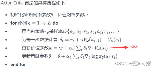
A2C相比于REINFORCE采用MC方法直接预估Q函数，A2C性能稳定，具有较小的方差。

3.2 Code

import gym
import torch
import torch.nn as nn
import torch.nn.functional as F
import numpy as np
import matplotlib.pyplot as plt
import rl_utils

首先定义策略网络PolicyNet（同REINFORCE）用于动作选择。

class PolicyNet(nn.Module):
    def __init__(self, state_dim, hidden_dim, action_dim):
        super(PolicyNet, self).__init__()
        self.fc1 = nn.Linear(state_dim, hidden_dim)
        self.fc2 = nn.Linear(hidden_dim, action_dim)
        
    def forward(self, x):
        x = F.relu(self.fc1(x))
        return F.softmax(self.fc2(x), dim=1) # dim=1，对每行使用softmax

接着定义价值网络ValueNet用于评估状态价值评估。

class ValueNet(nn.Module):
    def __init__(self, state_dim, hidden_dim):
        super(ValueNet, self).__init__()
        self.fc1 = nn.Linear(state_dim, hidden_dim)
        self.fc2 = nn.Linear(hidden_dim, 1)
    
    def forward(self, x):
        x = F.relu(self.fc1(x))
        return self.fc2(x)

Actor-Critic由actor和critic两个网络组成，critic用于输出状态的价值，actor选择动作并根据critic提供的价值优化策略。因此动作选取与REINFORCE相同，不同点在于策略优化部分。

class ActorCritic:
    def __init__(self, state_dim, hidden_dim, action_dim, actor_lr,
                critic_lr, gamma, device):
        self.actor = PolicyNet(state_dim, hidden_dim, action_dim).to(device)
        self.critic = ValueNet(state_dim, hidden_dim).to(device)
        self.actor_optimizer = torch.optim.Adam(self.actor.parameters(),
                                               lr = actor_lr)
        self.critic_optimizer = torch.optim.Adam(self.critic.parameters(),
                                                lr = critic_lr)
        self.gamma = gamma
        self.device = device
    
    # action selection，同REINFORCE    
    def take_action(self, state):
        state = torch.tensor([state], dtype=torch.float).to(self.device)
        probs = self.actor(state)
        action_dist = torch.distributions.Categorical(probs)
        action = action_dist.sample()
        return action.item()
    
    def update(self, transition_dict):
        states = torch.tensor(transition_dict['states'],
                             dtype=torch.float).to(self.device)
        actions = torch.tensor(transition_dict['actions']).view(-1,1).to(self.device)
        rewards = torch.tensor(transition_dict['rewards'],
                              dtype=torch.float).view(-1,1).to(self.device)
        next_states = torch.tensor(transition_dict['next_states'],
                              dtype=torch.float).to(self.device)
        dones = torch.tensor(transition_dict['dones'],
                            dtype=torch.float).view(-1,1).to(self.device)
        
#       TD-Target = r + v(s_{t+1})
        td_target = rewards + self.gamma * self.critic(next_states) * (1-dones)
#       TD-Error
        td_error = td_target - self.critic(states)
        log_probs = torch.log(self.actor(states).gather(1, actions))
        
        actor_loss = torch.mean(-log_probs * td_error.detach())
        critic_loss = torch.mean(F.mse_loss(self.critic(states), td_target.detach()))
        
        self.actor_optimizer.zero_grad()
        self.critic_optimizer.zero_grad()
        actor_loss.backward()
        critic_loss.backward()
        self.actor_optimizer.step()
        self.critic_optimizer.step()

根据策略梯度与价值函数损失优化策略和价值网络。