Keras深度学习实战(33)——基于LSTM的序列预测模型
Keras深度学习实战(33)——基于LSTM的序列预测模型
-
- 0. 前言
- 1. 序列学习任务
-
- 1.1 命名实体提取
- 1.2 文本摘要
- 1.3 机器翻译
- 2. 从输出网络返回输出序列
-
- 2.1 传统模型体系结构
- 2.2 返回每个时间戳的网络中间状态序列
- 2.3 使用双向 LSTM 网络
- 小结
- 系列链接
0. 前言
在《长短时记忆网络》一节中,我们了解到长短时记忆网络 (Long Short Term Memory, LSTM) 可以返回最后一个时间戳的结果,即输出为一维数据,而多对多神经网络架构输出为多个维度,其中每个维度对应一个输出,而非多个类别的 softmax 激活函数值。例如,在股价预测中,我们可以使用多对多神经网络架构预测未来 5 天的股价,而不仅是下一个交易日的股价;或者,对于给定的输入序列组合,我们不仅要预测下一个单词,而是要预测接下来 5 个单词的序列。在这类情况下,我们构建神经网络模型的方式有所不同。在本节中,我们将构建 LSTM 模型以提取不同时间戳的输出。
1. 序列学习任务
1.1 命名实体提取
命名实体就是人名、机构名、地名以及其他所有以名称为标识的实体。在命名实体提取中,我们试图为句子中存在的每个单词分配一个标签——标识其是否与命名实体有关。因此,命名实体提取是输入单词和输出类别之间的一对一映射的问题,标识单词是否为命名实体。尽管它是输入和输出之间的一对一映射,但在某些情况下,在确定输入单词是否为命名实体时,其周围的单词起着重要作用。例如,单词 new 本身可能不是命名实体。但是,如果 new 后伴随着 york,那么 new york 是一个命名实体。因此,即使在大多数情况下,输入和输出之间可能存在一对一的映射关系,但是输入时间戳在确定单词是否为命名实体中也起着重要作用。
这是一个序列返回问题,因为我们根据输入单词序列来分配命名实体的输出序列。因此,这是一个输入与输出之间一对一映射问题,并且单词周围时间戳的输入在确定输出时起着关键作用。因此,我们需要时间戳的两个方向上的单词都可以修正输出,此时双向 LSTM (bidirectional LSTM, BiLSTM) 就派上用场了。
BiLSTM 的体系结构如下所示:
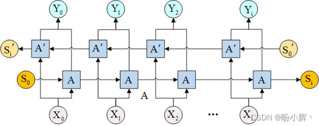
在上图中,我们修改了传统的 LSTM,使输入也以相反的方向相互连接,从而确保信息在两个方向上流动。我们将在后续学习中了解有关 BiLSTM 如何工作的更多信息。
1.2 文本摘要
文本摘要任务通常只有在处理完成整个输入语句之后,才能从文本中生成摘要。这要求将所有输入编码为一个向量,然后根据输入的编码向量生成输出。此外,鉴于文本中给定的单词序列有多个输出单词,因此它是一个多输出问题。常见的文本摘要模型如下所示:
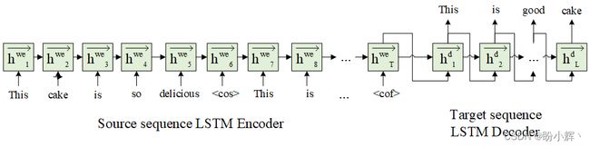
在以上体系结构中,我们利用所有输入文本编码,在输入序列的结尾字处生成结果向量,并将该编码向量作为输入传递给解码器序列。
1.3 机器翻译
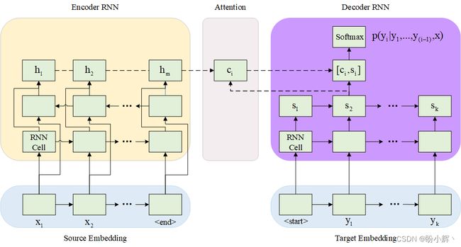
在以上场景中,我们将输入编码为一个向量,并希望该向量包含输入单词的顺序信息。我们通过在神经网络中引入注意力机制,使网络能够根据我们正在解码的单词的位置为位于给定位置的输入单词分配不同的权重。例如,如果源单词和目标单词对齐方式相似,即两种语言的词序相似,那么源语言开头的词对目标语言的最后一个词影响很小,但对确定目标语言中的第一个词有较大影响。
注意机制如下,注意力 (Attention) 向量受输入编码向量和输出值隐藏状态的影响:
2. 从输出网络返回输出序列
我们已经知道有多种方法可以设计网络以生成输出序列。在本节中,我们将学习利用编码器-解码器架构生成输出,以及有关示例数据集上输入到输出网络的一对一映射,以便深入了解编码器-解码器架构的工作原理。
2.1 传统模型体系结构
(1) 我们定义一个输入序列和一个对应的输出序列:
import numpy as np

input_data = np.array([[1,2],[3,4]])
output_data = np.array([[3,4],[5,6]])
我们定义的输入中有两个时间戳,并且给出了相应的输出。
(2) 我们首先定义传统模型体系结构,并使用函数式 API 提取输出、检查中间层状态:
from keras.layers import Input, LSTM, Dense
from keras import Model

# 定义模型
inputs1 = Input(shape=(2,1))
lstm1 = LSTM(1, activation = 'tanh', return_sequences=False,recurrent_activation='sigmoid')(inputs1)
out= Dense(2, activation='linear')(lstm1)
model = Model(inputs=inputs1, outputs=out)
model.summary()

model.compile(optimizer='adam',loss='mean_squared_error')
model.fit(input_data.reshape(2,2,1), output_data, epochs=50)
在以上代码中,输入 LSTM 的数据具有以下形状 (batch_size, time steps, features per time step),且 LSTM 不返回网络中间状态,即参数 return_sequences=False,并在 LSTM 层后添加全连接层,模型的输出为二维向量。模型架构简要信息如下:
Model: "functional_1"
_________________________________________________________________
Layer (type)                 Output Shape              Param #
=================================================================
input_1 (InputLayer)         [(None, 2, 1)]            0
_________________________________________________________________
lstm (LSTM)                  (None, 1)                 12
_________________________________________________________________
dense (Dense)                (None, 2)                 4
=================================================================
Total params: 16
Trainable params: 16
Non-trainable params: 0
_________________________________________________________________
(3) 接下来,编译并模型拟合:
model.compile(optimizer='adam',loss='mean_squared_error')
model.fit(input_data.reshape(2,2,1), output_data, epochs=50)
# 使用模型预测输出
print(model.predict(input_data[0].reshape(1,2,1)))
# [[0.05298579 0.03891079]]
(4) 有了输出之后,我们计算网络前向传播进行验证,验证过程与我们在介绍 LSTM 时使用的代码完全相同:
input_t0 = input_data[0][0]
cell_state0 = 0
forget0 = input_t0*model.get_weights()[0][0][1] + model.get_weights()[2][1]
forget1 = 1/(1+np.exp(-(forget0)))
cell_state1 = forget1 * cell_state0
input_t0_1 = input_t0*model.get_weights()[0][0][0] + model.get_weights()[2][0]
input_t0_2 = 1/(1+np.exp(-(input_t0_1)))
input_t0_cell1 = input_t0*model.get_weights()[0][0][2] + model.get_weights()[2][2]
input_t0_cell2 = np.tanh(input_t0_cell1)
input_t0_cell3 = input_t0_cell2*input_t0_2
input_t0_cell4 = input_t0_cell3 + cell_state1
output_t0_1 = input_t0*model.get_weights()[0][0][3] + model.get_weights()[2][3]
output_t0_2 = 1/(1+np.exp(-output_t0_1))
hidden_layer_1 = np.tanh(input_t0_cell4)*output_t0_2

input_t1 = input_data[0][1]
cell_state1 = input_t0_cell4
forget21 = hidden_layer_1*model.get_weights()[1][0][1] + model.get_weights()[2][1] + input_t1*model.get_weights()[0][0][1]
forget_22 = 1/(1+np.exp(-(forget21)))
cell_state2 = cell_state1 * forget_22
input_t1_1 = input_t1*model.get_weights()[0][0][0] + model.get_weights()[2][0] + hidden_layer_1*model.get_weights()[1][0][0]
input_t1_2 = 1/(1+np.exp(-(input_t1_1)))
input_t1_cell1 = input_t1*model.get_weights()[0][0][2] + model.get_weights()[2][2]+ hidden_layer_1*model.get_weights()[1][0][2]
input_t1_cell2 = np.tanh(input_t1_cell1)
input_t1_cell3 = input_t1_cell2*input_t1_2
input_t1_cell4 = input_t1_cell3 + cell_state2
output_t1_1 = input_t1*model.get_weights()[0][0][3] + model.get_weights()[2][3]+ hidden_layer_1*model.get_weights()[1][0][3]
output_t1_2 = 1/(1+np.exp(-output_t1_1))
hidden_layer_2 = np.tanh(input_t1_cell4)*output_t1_2
final_output = hidden_layer_2 * model.get_weights()[3][0] + model.get_weights()[4]

print(final_output)
final_output 的输出结果如下,其与使用模型 predict 方法预测的结果完全相同:
[0.05298579 0.03891079]
以这种方式生成输出的缺点之一是,在时间步长 1 的输出肯定不依赖于时间步长 2 的情况下,当我们从时间戳 2 获取输出时,由于其融合了时间戳 1 的网络中间状态和时间戳 2 的输入,因此模型很难分离时间戳 2 对时间戳 1 的影响。 我们可以通过从每个时间戳提取网络中间状态值,然后将其传递给全连接层来解决此问题。
2.2 返回每个时间戳的网络中间状态序列
(1) 接下来,我们将了解如何返回每个时间戳的网络中间状态值序列。
inputs1 = Input(shape=(2,1))
lstm1 = LSTM(1, activation = 'tanh', return_sequences=True, recurrent_activation='sigmoid')(inputs1)
out= Dense(1, activation='linear')(lstm1)
model = Model(inputs=inputs1, outputs=out)
model.summary()
在 LSTM 层中将 return_sequences 参数的值更改为 True,全连接层中输出维度为 1,模型架构简要信息如下:
Model: "functional_1"
_________________________________________________________________
Layer (type)                 Output Shape              Param #
=================================================================
input_1 (InputLayer)         [(None, 2, 1)]            0
_________________________________________________________________
lstm (LSTM)                  (None, 2, 1)              12
_________________________________________________________________
dense (Dense)                (None, 2, 1)              2
=================================================================
Total params: 14
Trainable params: 14
Non-trainable params: 0
_________________________________________________________________
由于我们提取了每个时间戳的网络中间状态输出,因此 LSTM 的输出形状为 (batch size, time steps, 1)。此外,由于每个时间戳都有将 LSTM 输出连接到最终输出的全连接层,因此输出形状与 LSTM 输出形状相同。
(2) 编译并拟合模型,并使用训练后的模型对输入值进行预测:
model.compile(optimizer='adam',loss='mean_squared_error')
model.fit(input_data.reshape(2,2,1), output_data.reshape(2,2,1),epochs=50)

print(model.predict(input_data[0].reshape(1,2,1)))
预测值结果输出如下:
[[[-0.05737699]
  [-0.08663369]]]
(3) 接下来,与上一小节类似,我们通过提取权重计算输入的前向传播过程来验证模型预测结果。首先,提取第 1 个时间戳的输出:
input_t0 = input_data[0][0]
cell_state0 = 0
forget0 = input_t0*model.get_weights()[0][0][1] + model.get_weights()[2][1]
forget1 = 1/(1+np.exp(-(forget0)))
cell_state1 = forget1 * cell_state0
input_t0_1 = input_t0*model.get_weights()[0][0][0] + model.get_weights()[2][0]
input_t0_2 = 1/(1+np.exp(-(input_t0_1)))
input_t0_cell1 = input_t0*model.get_weights()[0][0][2] + model.get_weights()[2][2]
input_t0_cell2 = np.tanh(input_t0_cell1)
input_t0_cell3 = input_t0_cell2*input_t0_2
input_t0_cell4 = input_t0_cell3 + cell_state1
output_t0_1 = input_t0*model.get_weights()[0][0][3] + model.get_weights()[2][3]
output_t0_2 = 1/(1+np.exp(-output_t0_1))
hidden_layer_1 = np.tanh(input_t0_cell4)*output_t0_2
final_output_1 = hidden_layer_1 * model.get_weights()[3][0] + model.get_weights()[4]
print(final_output_1)
# [-0.05737697]
可以看到,final_output_1 值与模型预测值的第一个维度完全相同。同样,我们继续验证第 2 个时间戳的输出,可以看到,计算结果同样与 model.predict 的返回结果相同:
input_t1 = input_data[0][1]
cell_state1 = input_t0_cell4
forget21 = hidden_layer_1*model.get_weights()[1][0][1] + model.get_weights()[2][1] + input_t1*model.get_weights()[0][0][1]
forget_22 = 1/(1+np.exp(-(forget21)))
cell_state2 = cell_state1 * forget_22
input_t1_1 = input_t1*model.get_weights()[0][0][0] + model.get_weights()[2][0] + hidden_layer_1*model.get_weights()[1][0][0]
input_t1_2 = 1/(1+np.exp(-(input_t1_1)))
input_t1_cell1 = input_t1*model.get_weights()[0][0][2] + model.get_weights()[2][2]+ hidden_layer_1*model.get_weights()[1][0][2]
input_t1_cell2 = np.tanh(input_t1_cell1)
input_t1_cell3 = input_t1_cell2*input_t1_2
input_t1_cell4 = input_t1_cell3 + cell_state2
output_t1_1 = input_t1*model.get_weights()[0][0][3] + model.get_weights()[2][3]+ hidden_layer_1*model.get_weights()[1][0][3]
output_t1_2 = 1/(1+np.exp(-output_t1_1))
hidden_layer_2 = np.tanh(input_t1_cell4)*output_t1_2
final_output_2 = hidden_layer_2 * model.get_weights()[3][0] + model.get_weights()[4]
print(final_output_2)
了解了 LSTM 层中的 return_sequences 参数,接下来,我们继续学习另一个称为 return_state 的参数。我们知道 LSTM 网络的两个输出是每个时间戳的 LSTM 输出值和单元状态值,return_state 用于提取 LSTM 层中的单元状态值。当输入文本被编码为矢量时,提取单元状态非常有用,我们不仅可以将编码向量传递给解码器网络,还将编码器的单元状态传递给解码器网络。
(4) 接下来,我们了解 return_state 的工作原理,我们只需要了解每个时间戳的单元状态是如何生成的。在实践中,我们可以直接使用 LSTM 输出值和单元状态值作为解码器的输入:
inputs1 = Input(shape=(2,1))
lstm1,state_h,state_c = LSTM(1, activation = 'tanh', return_sequences=True, return_state = True, recurrent_activation='sigmoid')(inputs1)
model = Model(inputs=inputs1, outputs=[lstm1, state_h, state_c])
model.summary()
在以上代码中,我们将 return_state 参数设置为 True,此时 LSTM 的输出如下:
lstm1:每个时间戳的网络输出state_h:最后1个时间戳的网络输出state_c:最后1个时间戳的单元状态
(5) 编译并拟合模型,然后使用训练后的模型进行预测:
model.compile(optimizer='adam',loss='mean_squared_error')
model.fit(input_data.reshape(2,2,1), output_data.reshape(2,2,1),epochs=50)

print(model.predict(input_data[0].reshape(1,2,1)))
网络预测输出值如下:
[array([[[0.05678726],
        [0.1279237 ]]], dtype=float32), array([[0.1279237]], dtype=float32), array([[0.22134428]], dtype=float32)]
可以看到有三个输出数组,如前所述,分别对应每个时间戳的网络输出序列、LSTM 最终输出值和最终单元状态。
(6) 接下来,我们同样验证 LSTM 的这些输出:
input_t0 = input_data[0][0]
cell_state0 = 0
forget0 = input_t0*model.get_weights()[0][0][1] + model.get_weights()[2][1]
forget1 = 1/(1+np.exp(-(forget0)))
cell_state1 = forget1 * cell_state0
input_t0_1 = input_t0*model.get_weights()[0][0][0] + model.get_weights()[2][0]
input_t0_2 = 1/(1+np.exp(-(input_t0_1)))
input_t0_cell1 = input_t0*model.get_weights()[0][0][2] + model.get_weights()[2][2]
input_t0_cell2 = np.tanh(input_t0_cell1)
input_t0_cell3 = input_t0_cell2*input_t0_2
input_t0_cell4 = input_t0_cell3 + cell_state1
output_t0_1 = input_t0*model.get_weights()[0][0][3] + model.get_weights()[2][3]
output_t0_2 = 1/(1+np.exp(-output_t0_1))
hidden_layer_1 = np.tanh(input_t0_cell4)*output_t0_2
print(hidden_layer_1)
hidden_layer_1 的值为 LSTM 在时间戳 1 时的输出:
0.05678726552767216
接下来,我们继续验证其它输出:
input_t1 = input_data[0][1]
cell_state1 = input_t0_cell4
forget21 = hidden_layer_1*model.get_weights()[1][0][1] + model.get_weights()[2][1] + input_t1*model.get_weights()[0][0][1]
forget_22 = 1/(1+np.exp(-(forget21)))
cell_state2 = cell_state1 * forget_22
input_t1_1 = input_t1*model.get_weights()[0][0][0] + model.get_weights()[2][0] + hidden_layer_1*model.get_weights()[1][0][0]
input_t1_2 = 1/(1+np.exp(-(input_t1_1)))
input_t1_cell1 = input_t1*model.get_weights()[0][0][2] + model.get_weights()[2][2]+ hidden_layer_1*model.get_weights()[1][0][2]
input_t1_cell2 = np.tanh(input_t1_cell1)
input_t1_cell3 = input_t1_cell2*input_t1_2
input_t1_cell4 = input_t1_cell3 + cell_state2
output_t1_1 = input_t1*model.get_weights()[0][0][3] + model.get_weights()[2][3]+ hidden_layer_1*model.get_weights()[1][0][3]
output_t1_2 = 1/(1+np.exp(-output_t1_1))
hidden_layer_2 = np.tanh(input_t1_cell4)*output_t1_2
print(hidden_layer_2, input_t1_cell4)
可以看到输出结果与使用预测函数 predict 得到的结果完全相同:
0.12792369406644594 0.22134428173524104
2.3 使用双向 LSTM 网络
(1) 接下来,我们使用双向 LSTM 网络,从两侧计算 LSTM 网络在每一时间戳的输出值时需要将它们合并在一起:
from keras.layers import Bidirectional

inputs1 = Input(shape=(2,1))
lstm1,state_fh,state_fc,state_bh,state_bc = Bidirectional(LSTM(1, activation = 'tanh', return_sequences=True, return_state = True, recurrent_initializer='Zeros',recurrent_activation='sigmoid'))(inputs1)
model = Model(inputs=inputs1, outputs=[lstm1, state_fh,state_fc,state_bh,state_bc])
model.summary()

model.compile(optimizer='adam',loss='mean_squared_error')
model.fit(input_data.reshape(2,2,1), output_data.reshape(2,2,1),epochs=50)
(2) 在双向 LSTM 中,最终 LSTM 网络有两个输出,一个是从左到右考虑输入时间戳,另一个是从右到左考虑输入时间戳;同理可得,我们将有两个单元状态。接下来,我们同样验证双向 LSTM 的输出:
print(model.predict(input_data[0].reshape(1,2,1)))

input_t0 = input_data[0][0]
cell_state0 = 0
forget0 = input_t0*model.get_weights()[0][0][1] + model.get_weights()[2][1]
forget1 = 1/(1+np.exp(-(forget0)))
cell_state1 = forget1 * cell_state0
input_t0_1 = input_t0*model.get_weights()[0][0][0] + model.get_weights()[2][0]
input_t0_2 = 1/(1+np.exp(-(input_t0_1)))
input_t0_cell1 = input_t0*model.get_weights()[0][0][2] + model.get_weights()[2][2]
input_t0_cell2 = np.tanh(input_t0_cell1)
input_t0_cell3 = input_t0_cell2*input_t0_2
input_t0_cell4 = input_t0_cell3 + cell_state1
output_t0_1 = input_t0*model.get_weights()[0][0][3] + model.get_weights()[2][3]
output_t0_2 = 1/(1+np.exp(-output_t0_1))
hidden_layer_1 = np.tanh(input_t0_cell4)*output_t0_2
print(hidden_layer_1)

input_t1 = input_data[0][1]
cell_state1 = input_t0_cell4
forget21 = hidden_layer_1*model.get_weights()[1][0][1] + model.get_weights()[2][1] + input_t1*model.get_weights()[0][0][1]
forget_22 = 1/(1+np.exp(-(forget21)))
cell_state2 = cell_state1 * forget_22
input_t1_1 = input_t1*model.get_weights()[0][0][0] + model.get_weights()[2][0] + hidden_layer_1*model.get_weights()[1][0][0]
input_t1_2 = 1/(1+np.exp(-(input_t1_1)))
input_t1_cell1 = input_t1*model.get_weights()[0][0][2] + model.get_weights()[2][2]+ hidden_layer_1*model.get_weights()[1][0][2]
input_t1_cell2 = np.tanh(input_t1_cell1)
input_t1_cell3 = input_t1_cell2*input_t1_2
input_t1_cell4 = input_t1_cell3 + cell_state2
output_t1_1 = input_t1*model.get_weights()[0][0][3] + model.get_weights()[2][3]+ hidden_layer_1*model.get_weights()[1][0][3]
output_t1_2 = 1/(1+np.exp(-output_t1_1))
hidden_layer_2 = np.tanh(input_t1_cell4)*output_t1_2
print(hidden_layer_2, input_t1_cell4)

input_t0 = input_data[0][1]
cell_state0 = 0
forget0 = input_t0*model.get_weights()[3][0][1] + model.get_weights()[5][1]
forget1 = 1/(1+np.exp(-(forget0)))
cell_state1 = forget1 * cell_state0
input_t0_1 = input_t0*model.get_weights()[3][0][0] + model.get_weights()[5][0]
input_t0_2 = 1/(1+np.exp(-(input_t0_1)))
input_t0_cell1 = input_t0*model.get_weights()[3][0][2] + model.get_weights()[5][2]
input_t0_cell2 = np.tanh(input_t0_cell1)
input_t0_cell3 = input_t0_cell2*input_t0_2
input_t0_cell4 = input_t0_cell3 + cell_state1
output_t0_1 = input_t0*model.get_weights()[3][0][3] + model.get_weights()[5][3]
output_t0_2 = 1/(1+np.exp(-output_t0_1))
hidden_layer_1 = np.tanh(input_t0_cell4)*output_t0_2
print(hidden_layer_1)

input_t1 = input_data[0][0]
cell_state1 = input_t0_cell4
forget21 = hidden_layer_1*model.get_weights()[4][0][1] + model.get_weights()[5][1] + input_t1*model.get_weights()[3][0][1]
forget_22 = 1/(1+np.exp(-(forget21)))
cell_state2 = cell_state1 * forget_22
input_t1_1 = input_t1*model.get_weights()[3][0][0] + model.get_weights()[5][0] + hidden_layer_1*model.get_weights()[4][0][0]
input_t1_2 = 1/(1+np.exp(-(input_t1_1)))
input_t1_cell1 = input_t1*model.get_weights()[3][0][2] + model.get_weights()[5][2]+ hidden_layer_1*model.get_weights()[4][0][2]
input_t1_cell2 = np.tanh(input_t1_cell1)
input_t1_cell3 = input_t1_cell2*input_t1_2
input_t1_cell4 = input_t1_cell3 + cell_state2
output_t1_1 = input_t1*model.get_weights()[3][0][3] + model.get_weights()[5][3]+ hidden_layer_1*model.get_weights()[4][0][3]
output_t1_2 = 1/(1+np.exp(-output_t1_1))
hidden_layer_2 = np.tanh(input_t1_cell4)*output_t1_2
print(hidden_layer_2, input_t1_cell4)
得到的输出结果如下所示,可以看到通过前向计算得到的网络输出与使用 predict 方法得到的网络预测值完全相同:
[array([[[0.06926353, 0.22431403],
        [0.20269555, 0.09108724]]], dtype=float32), array([[0.20269555]], dtype=float32), array([[0.29688594]], dtype=float32), array([[0.22431403]], dtype=float32), array([[1.0147126]], dtype=float32)]
0.06926351566779305
0.2026955582957684 0.2968859343446881
0.09108724342304113
0.2243140321504562 1.0147124600076545
小结
近几年,深度学习飞速发展,基于该技术的方法在多个自然语言处理任务上取得了良好效果。长短时记忆网络 (Long Short Term Memory, LSTM) 具有优异的序列学习能力,这使其成为目前序列预测领域的一个研究热点。本文基于 LSTM 研究各类不同模型的序列预测问题,包括一对一架构以及多对多架构,并且通过实战验证了不同架构的输出结果。
系列链接
Keras深度学习实战(1)——神经网络基础与模型训练过程详解
Keras深度学习实战(2)——使用Keras构建神经网络
Keras深度学习实战(3)——神经网络性能优化技术
Keras深度学习实战(4)——深度学习中常用激活函数和损失函数详解
Keras深度学习实战(5)——批归一化详解
Keras深度学习实战(6)——深度学习过拟合问题及解决方法
Keras深度学习实战(7)——卷积神经网络详解与实现
Keras深度学习实战(8)——使用数据增强提高神经网络性能
Keras深度学习实战(9)——卷积神经网络的局限性
Keras深度学习实战(10)——迁移学习详解
Keras深度学习实战(11)——可视化神经网络中间层输出
Keras深度学习实战(12)——面部特征点检测
Keras深度学习实战(13)——目标检测基础详解
Keras深度学习实战(14)——从零开始实现R-CNN目标检测
Keras深度学习实战(15)——从零开始实现YOLO目标检测
Keras深度学习实战(16)——自编码器详解
Keras深度学习实战(17)——使用U-Net架构进行图像分割
Keras深度学习实战(18)——语义分割详解
Keras深度学习实战(19)——使用对抗攻击生成可欺骗神经网络的图像
Keras深度学习实战(20)——DeepDream模型详解
Keras深度学习实战(21)——神经风格迁移详解
Keras深度学习实战(22)——生成对抗网络详解与实现
Keras深度学习实战(23)——DCGAN详解与实现
Keras深度学习实战(24)——从零开始构建单词向量
Keras深度学习实战(25)——使用skip-gram和CBOW模型构建单词向量
Keras深度学习实战(26)——文档向量详解
Keras深度学习实战(27)——循环神经详解与实现
Keras深度学习实战(28)——利用单词向量构建情感分析模型
Keras深度学习实战(29)——长短时记忆网络详解与实现
Keras深度学习实战(30)——使用文本生成模型进行文学创作
Keras深度学习实战(31)——构建电影推荐系统
Keras深度学习实战(32)——基于LSTM预测股价