PINN深度学习求解微分方程系列三:求解burger方程逆问题
下面我将介绍内嵌物理知识神经网络(PINN)求解微分方程。首先介绍PINN基本方法,并基于Pytorch的PINN求解框架实现求解含时间项的一维burger方程。
内嵌物理知识神经网络(PINN)入门及相关论文
深度学习求解微分方程系列一:PINN求解框架(Poisson 1d)
深度学习求解微分方程系列二:PINN求解burger方程正问题
深度学习求解微分方程系列三:PINN求解burger方程逆问题
深度学习求解微分方程系列四:基于自适应激活函数PINN求解burger方程逆问题
1.PINN简介
神经网络作为一种强大的信息处理工具在计算机视觉、生物医学、 油气工程领域得到广泛应用, 引发多领域技术变革.。深度学习网络具有非常强的学习能力, 不仅能发现物理规律, 还能求解偏微分方程.。近年来,基于深度学习的偏微分方程求解已是研究新热点。内嵌物理知识神经网络(PINN)是一种科学机器在传统数值领域的应用方法,能够用于解决与偏微分方程 (PDE) 相关的各种问题,包括方程求解、参数反演、模型发现、控制与优化等。
2.PINN方法
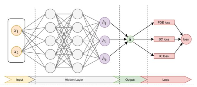
PINN的主要思想如图1,先构建一个输出结果为 u ^ \hat{u} u^的神经网络,将其作为PDE解的代理模型,将PDE信息作为约束,编码到神经网络损失函数中进行训练。损失函数主要包括4部分:偏微分结构损失(PDE loss),边值条件损失(BC loss)、初值条件损失(IC loss)以及真实数据条件损失(Data loss)。
特别的,考虑下面这个的PDE问题,其中PDE的解 u ( x ) u(x) u(x)在 Ω ⊂ R d \Omega \subset \mathbb{R}^{d} Ω⊂Rd定义,其中 x = ( x 1 , … , x d ) \mathbf{x}=\left(x_{1}, \ldots, x_{d}\right) x=(x1,…,xd):
f ( x ; ∂ u ∂ x 1 , … , ∂ u ∂ x d ; ∂ 2 u ∂ x 1 ∂ x 1 , … , ∂ 2 u ∂ x 1 ∂ x d ) = 0 , x ∈ Ω f\left(\mathbf{x} ; \frac{\partial u}{\partial x_{1}}, \ldots, \frac{\partial u}{\partial x_{d}} ; \frac{\partial^{2} u}{\partial x_{1} \partial x_{1}}, \ldots, \frac{\partial^{2} u}{\partial x_{1} \partial x_{d}} \right)=0, \quad \mathbf{x} \in \Omega f(x;∂x1∂u,…,∂xd∂u;∂x1∂x1∂2u,…,∂x1∂xd∂2u)=0,x∈Ω
同时,满足下面的边界
B ( u , x ) = 0 on ∂ Ω \mathcal{B}(u, \mathbf{x})=0 \quad \text { on } \quad \partial \Omega B(u,x)=0 on ∂Ω
PINN求解过程主要包括:
- 第一步,首先定义D层全连接层的神经网络模型:
N Θ : = L D ∘ σ ∘ L D − 1 ∘ σ ∘ ⋯ ∘ σ ∘ L 1 N_{\Theta}:=L_D \circ \sigma \circ L_{D-1} \circ \sigma \circ \cdots \circ \sigma \circ L_1 NΘ:=LD∘σ∘LD−1∘σ∘⋯∘σ∘L1
式中:
L 1 ( x ) : = W 1 x + b 1 , W 1 ∈ R d 1 × d , b 1 ∈ R d 1 L i ( x ) : = W i x + b i , W i ∈ R d i × d i − 1 , b i ∈ R d i , ∀ i = 2 , 3 , ⋯ D − 1 , L D ( x ) : = W D x + b D , W D ∈ R N × d D − 1 , b D ∈ R N . \begin{aligned} L_1(x) &:=W_1 x+b_1, \quad W_1 \in \mathbb{R}^{d_1 \times d}, b_1 \in \mathbb{R}^{d_1} \\ L_i(x) &:=W_i x+b_i, \quad W_i \in \mathbb{R}^{d_i \times d_{i-1}}, b_i \in \mathbb{R}^{d_i}, \forall i=2,3, \cdots D-1, \\ L_D(x) &:=W_D x+b_D, \quad W_D \in \mathbb{R}^{N \times d_{D-1}}, b_D \in \mathbb{R}^N . \end{aligned} L1(x)Li(x)LD(x):=W1x+b1,W1∈Rd1×d,b1∈Rd1:=Wix+bi,Wi∈Rdi×di−1,bi∈Rdi,∀i=2,3,⋯D−1,:=WDx+bD,WD∈RN×dD−1,bD∈RN.
以及 σ \sigma σ 为激活函数, W W W 和 b b b 为权重和偏差参数。 - 第二步,为了衡量神经网络 u ^ \hat{u} u^和约束之间的差异,考虑损失函数定义:
L ( θ ) = w f L P D E ( θ ; T f ) + w i L I C ( θ ; T i ) + w b L B C ( θ , ; T b ) + w d L D a t a ( θ , ; T d a t a ) \mathcal{L}\left(\boldsymbol{\theta}\right)=w_{f} \mathcal{L}_{PDE}\left(\boldsymbol{\theta}; \mathcal{T}_{f}\right)+w_{i} \mathcal{L}_{IC}\left(\boldsymbol{\theta} ; \mathcal{T}_{i}\right)+w_{b} \mathcal{L}_{BC}\left(\boldsymbol{\theta},; \mathcal{T}_{b}\right)+w_{d} \mathcal{L}_{Data}\left(\boldsymbol{\theta},; \mathcal{T}_{data}\right) L(θ)=wfLPDE(θ;Tf)+wiLIC(θ;Ti)+wbLBC(θ,;Tb)+wdLData(θ,;Tdata)
式中:
L P D E ( θ ; T f ) = 1 ∣ T f ∣ ∑ x ∈ T f ∥ f ( x ; ∂ u ^ ∂ x 1 , … , ∂ u ^ ∂ x d ; ∂ 2 u ^ ∂ x 1 ∂ x 1 , … , ∂ 2 u ^ ∂ x 1 ∂ x d ) ∥ 2 2 L I C ( θ ; T i ) = 1 ∣ T i ∣ ∑ x ∈ T i ∥ u ^ ( x ) − u ( x ) ∥ 2 2 L B C ( θ ; T b ) = 1 ∣ T b ∣ ∑ x ∈ T b ∥ B ( u ^ , x ) ∥ 2 2 L D a t a ( θ ; T d a t a ) = 1 ∣ T d a t a ∣ ∑ x ∈ T d a t a ∥ u ^ ( x ) − u ( x ) ∥ 2 2 \begin{aligned} \mathcal{L}_{PDE}\left(\boldsymbol{\theta} ; \mathcal{T}_{f}\right) &=\frac{1}{\left|\mathcal{T}_{f}\right|} \sum_{\mathbf{x} \in \mathcal{T}_{f}}\left\|f\left(\mathbf{x} ; \frac{\partial \hat{u}}{\partial x_{1}}, \ldots, \frac{\partial \hat{u}}{\partial x_{d}} ; \frac{\partial^{2} \hat{u}}{\partial x_{1} \partial x_{1}}, \ldots, \frac{\partial^{2} \hat{u}}{\partial x_{1} \partial x_{d}} \right)\right\|_{2}^{2} \\ \mathcal{L}_{IC}\left(\boldsymbol{\theta}; \mathcal{T}_{i}\right) &=\frac{1}{\left|\mathcal{T}_{i}\right|} \sum_{\mathbf{x} \in \mathcal{T}_{i}}\|\hat{u}(\mathbf{x})-u(\mathbf{x})\|_{2}^{2} \\ \mathcal{L}_{BC}\left(\boldsymbol{\theta}; \mathcal{T}_{b}\right) &=\frac{1}{\left|\mathcal{T}_{b}\right|} \sum_{\mathbf{x} \in \mathcal{T}_{b}}\|\mathcal{B}(\hat{u}, \mathbf{x})\|_{2}^{2}\\ \mathcal{L}_{Data}\left(\boldsymbol{\theta}; \mathcal{T}_{data}\right) &=\frac{1}{\left|\mathcal{T}_{data}\right|} \sum_{\mathbf{x} \in \mathcal{T}_{data}}\|\hat{u}(\mathbf{x})-u(\mathbf{x})\|_{2}^{2} \end{aligned} LPDE(θ;Tf)LIC(θ;Ti)LBC(θ;Tb)LData(θ;Tdata)=∣Tf∣1x∈Tf∑∥ ∥f(x;∂x1∂u^,…,∂xd∂u^;∂x1∂x1∂2u^,…,∂x1∂xd∂2u^)∥ ∥22=∣Ti∣1x∈Ti∑∥u^(x)−u(x)∥22=∣Tb∣1x∈Tb∑∥B(u^,x)∥22=∣Tdata∣1x∈Tdata∑∥u^(x)−u(x)∥22
w f w_{f} wf, w i w_{i} wi、 w b w_{b} wb和 w d w_{d} wd是权重。 T f \mathcal{T}_{f} Tf, T i \mathcal{T}_{i} Ti、 T b \mathcal{T}_{b} Tb和 T d a t a \mathcal{T}_{data} Tdata表示来自PDE,初值、边值以及真值的residual points。这里的 T f ⊂ Ω \mathcal{T}_{f} \subset \Omega Tf⊂Ω是一组预定义的点来衡量神经网络输出 u ^ \hat{u} u^与PDE的匹配程度。 - 最后,利用梯度优化算法最小化损失函数,直到找到满足预测精度的网络参数 KaTeX parse error: Undefined control sequence: \theat at position 1: \̲t̲h̲e̲a̲t̲^{*}。
值得注意的是,对于逆问题,即方程中的某些参数未知。若只知道PDE方程及边界条件,PDE参数未知,该逆问题为非定问题,所以必须要知道其他信息,如部分观测点 u u u 的值。在这种情况下,PINN做法可将方程中的参数作为未知变量,加到训练器中进行优化,损失函数包括Data loss。
3.求解问题定义——逆问题
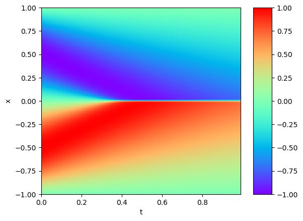
u t + u u x = v u x x , x ∈ [ − 1 , 1 ] , t > 0 u ( x , 0 ) = − sin ( π x ) u ( − 1 , t ) = u ( 1 , t ) = 0 \begin{aligned} u_t+u u_x &=v u_{x x}, x \in[-1,1], t>0 \\ u(x, 0) &=-\sin (\pi x) \\ u(-1, t) &=u(1, t)=0 \end{aligned} ut+uuxu(x,0)u(−1,t)=vuxx,x∈[−1,1],t>0=−sin(πx)=u(1,t)=0
式中:参数 v v v为未知参数,真实值为 v ∈ [ 0 , 0.1 / π ] v \in[0,0.1 / \pi] v∈[0,0.1/π]。数值解通过Hopf-Cole transformation获得,如图2。
任务要求:
- 该任务为已知边界条件和微分方程,但方程中参数未知,求解u 以及方程参数。
- 该问题典型逆问题,优化方程参数的反演问题。
4.Python求解代码
- 第一步,首先定义神经网络。这里和之前网络不同点主要在于,网络中增加了可训练参数 a。
class Net(nn.Module):
    def __init__(self, seq_net, name='MLP', activation=torch.tanh):
        super().__init__()
        self.features = OrderedDict()
        for i in range(len(seq_net) - 1):
            self.features['{}_{}'.format(name, i)] = nn.Linear(seq_net[i], seq_net[i + 1], bias=True)
        self.features = nn.ModuleDict(self.features)
        self.active = activation

        # initial_bias
        for m in self.modules():
            if isinstance(m, nn.Linear):
                nn.init.constant_(m.bias, 0)

    def forward(self, x):
        # x = x.view(-1, 2)
        length = len(self.features)
        i = 0
        for name, layer in self.features.items():
            x = layer(x)
            if i == length - 1: break
            i += 1
            x = self.active(x)
        return x
- 第二步,PINN求解框架,定义网络,采点构建损失函数,优化器优化损失函数。这里和深度学习求解微分方程系列二:PINN求解burger方程,不同点主要在于多了Data loss项,同时PDE未知参数被加入网络优化器中进行训练。
from net import Net
import os
# from Parser_PINN import get_parser
from math import pi
import scipy.io
import numpy as np
import torch
from torch.autograd import grad
from math import pi
import matplotlib.pyplot as plt

def d(f, x):
    return grad(f, x, grad_outputs=torch.ones_like(f), create_graph=True, only_inputs=True)[0]


def PDE(u, t, x, nu):
    return d(u, t) + u * d(u, x) - nu * d(d(u, x), x)


def Ground_true(xx):
    out = 0.7 * torch.sin(pi * xx[:, 0:1]) * torch.sin(pi * xx[:, 1:]) + \
          0.45 * torch.sin(1 * pi * xx[:, 0:1]) * torch.sin(2 * pi * xx[:, 1:]) - \
          0.23 * torch.sin(1 * pi * xx[:, 0:1]) * torch.sin(3 * pi * xx[:, 1:]) - \
          0.10 * torch.sin(2 * pi * xx[:, 0:1]) * torch.sin(1 * pi * xx[:, 1:]) + \
          0.95 * torch.sin(2 * pi * xx[:, 0:1]) * torch.sin(2 * pi * xx[:, 1:]) - \
          0.95 * torch.sin(2 * pi * xx[:, 0:1]) * torch.sin(3 * pi * xx[:, 1:]) + \
          0.95 * torch.sin(3 * pi * xx[:, 0:1]) * torch.sin(1 * pi * xx[:, 1:]) - \
          0.95 * torch.sin(3 * pi * xx[:, 0:1]) * torch.sin(2 * pi * xx[:, 1:]) + \
          0.95 * torch.sin(3 * pi * xx[:, 0:1]) * torch.sin(3 * pi * xx[:, 1:])

    return out

def train():

    t_left, t_right = 0., 1.
    x_left, x_right = -1., 1.
    lr = 0.001
    epochs = 60000
    n_f, n_b_1,n_b_2 = 10000, 400, 400
    N_train = 10000

    os.environ['CUDA_VISIBLE_DEVICES'] = '0'
    device = torch.device('cuda:0') if torch.cuda.is_available() else torch.cuda('cpu')

    PINN = Net(seq_net=[2, 20, 20, 20, 20, 20, 20, 1], activation=torch.tanh).to(device)
    optimizer = torch.optim.Adam(PINN.parameters(), lr)

    # Problem parameter initialization
    nu = np.array([0])
    nu = torch.from_numpy(nu).float().to(device).requires_grad_(True)
    nu.grad = torch.ones((1)).to(device)
    optimizer.add_param_group({'params': nu, 'lr': 0.00001})

    criterion = torch.nn.MSELoss()

    # data
    data = scipy.io.loadmat('Data/burgers_shock.mat')
    Exact = np.real(data['usol']).T
    t = data['t'].flatten()[:, None]
    x = data['x'].flatten()[:, None]
    X, T = np.meshgrid(x, t)
    s_shape = X.shape
    X_star = np.hstack((X.flatten()[:, None], T.flatten()[:, None]))  # Lay horizontally (25600, 2)
    X_star = X_star.astype(np.float32)  # first column represents x, second column represents t
    X_star = torch.from_numpy(X_star).cuda().requires_grad_(True)
    u_star = Exact.flatten()[:, None]
    u_star = u_star.astype(np.float32)
    u_star = torch.from_numpy(u_star).cuda().requires_grad_(True)


    # data

    N, T = 256, 100
    # print(X_star.shape)
    idx = np.random.choice(N * T, N_train, replace=False)
    x_train = X_star[idx, 0:1].requires_grad_(True)
    t_train = X_star[idx, 1:2].requires_grad_(True)
    u_train = u_star[idx]

    loss_history = []
    Lambda = []
    Loss_history = []
    test_loss = []

    for epoch in range(epochs):
        optimizer.zero_grad()
        # PDE residual
        t_f = ((t_left + t_right) / 2 + (t_right - t_left) *
               (torch.rand(size=(n_f, 1), dtype=torch.float, device=device) - 0.5)
               ).requires_grad_(True)

        x_f = ((x_left + x_right) / 2 + (x_right - x_left) *
               (torch.rand(size=(n_f, 1), dtype=torch.float, device=device) - 0.5)
               ).requires_grad_(True)
        u_f = PINN(torch.cat([t_f, x_f], dim=1))
        PDE_ = PDE(u_f, t_f, x_f, nu)
        mse_PDE = criterion(PDE_, torch.zeros_like(PDE_))

        # Boundary
        x_rand = ((x_left + x_right) / 2 + (x_right - x_left) *
                  (torch.rand(size=(n_b_1, 1), dtype=torch.float, device=device) - 0.5)
                  ).requires_grad_(True)
        t_b = (t_left * torch.ones_like(x_rand)
               ).requires_grad_(True)
        u_b_1 = PINN(torch.cat([t_b, x_rand], dim=1)) + torch.sin(pi * x_rand)

        t_rand = ((t_left + t_right) / 2 + (t_right - t_left) *
                  (torch.rand(size=(n_b_2, 1), dtype=torch.float, device=device) - 0.5)
                  ).requires_grad_(True)
        x_b_1 = (x_left * torch.ones_like(t_rand)
                 ).requires_grad_(True)
        x_b_2 = (x_right * torch.ones_like(t_rand)
                 ).requires_grad_(True)

        u_b_2 = PINN(torch.cat([t_rand, x_b_1], dim=1))
        u_b_3 = PINN(torch.cat([t_rand, x_b_2], dim=1))

        mse_BC_1 = criterion(u_b_1, torch.zeros_like(u_b_1))
        mse_BC_2 = criterion(u_b_2, torch.zeros_like(u_b_2))
        mse_BC_3 = criterion(u_b_3, torch.zeros_like(u_b_3))

        mse_BC = mse_BC_1 + mse_BC_2 + mse_BC_3

        # Data
        u_data = PINN(torch.cat([t_train, x_train], dim=1))
        mse_Data = criterion(u_data, u_train)

        # loss
        loss = 1 * mse_PDE + 1 * mse_BC + 1 * mse_Data

        # Pred loss
        x_pred = X_star[:, 0:1]
        t_pred = X_star[:, 1:2]
        u_pred = PINN(torch.cat([t_pred, x_pred], dim=1))
        mse_test = criterion(u_pred, u_star)

        loss_history.append([mse_PDE.item(), mse_BC.item(), mse_Data.item(), mse_test.item()])
        Lambda.append([nu.item()])
        Loss_history.append([loss.item()])
        test_loss.append([mse_test.item()])
        loss.backward(retain_graph=True)
        optimizer.step()

        if (epoch + 1) % 10000 == 0:
            print(
                'epoch:{:05d}, PDE: {:.08e}, BC: {:.08e},  loss: {:.08e}'.format(
                    epoch + 1, mse_PDE.item(), mse_BC.item(), loss.item()
                )
            )
            print('nu:{:.03e}'.format(nu.item()))

        if (epoch + 1) % 100 == 0:
            x_pred = X_star[:, 0:1]
            t_pred = X_star[:, 1:2]
            u_pred = PINN(torch.cat([t_pred, x_pred], dim=1))
            plt.pcolormesh(np.squeeze(t, axis=1), np.squeeze(x, axis=1),
                           u_pred.cpu().detach().numpy().reshape(s_shape).T, cmap='rainbow')
            cbar = plt.colorbar(pad=0.05, aspect=10)
            cbar.mappable.set_clim(-1, 1)
            plt.xticks([])
            plt.yticks([])
            plt.savefig('./result_plot/Burger1d_pred_{}.png'.format(epoch + 1), bbox_inches='tight', format='png')
            plt.show()

            plt.cla()
            mse_test = abs(u_pred - u_star)
            plt.pcolormesh(np.squeeze(t, axis=1), np.squeeze(x, axis=1),
                           mse_test.cpu().detach().numpy().reshape(s_shape).T, cmap='rainbow')
            cbar = plt.colorbar(pad=0.05, aspect=10)
            cbar.mappable.set_clim(0, 0.3)
            plt.xticks([])
            plt.yticks([])
            plt.savefig('./result_plot/Burger1d_error_{}.png'.format(epoch + 1), bbox_inches='tight', format='png')
            plt.show()


            #
            fig, ax = plt.subplots(1, 3, figsize=(12, 4))
            x_25 = x.astype(np.float32)
            x_25 = torch.from_numpy(x_25).cuda().requires_grad_(True)
            t_25 = (0.25 * torch.ones_like(x_25)).requires_grad_(True)
            u_25 = PINN(torch.cat([t_25, x_25], dim=1))
            ax[0].plot(x, Exact[25, :], 'b-', linewidth=2)
            ax[0].plot(x, u_25.reshape((-1, 1)).detach().cpu().numpy(), 'r-', linewidth=2, linestyle='--',
                       label='PINN', )
            ax[0].set_xlabel('x')
            ax[0].set_ylabel('u(t,x)')
            ax[0].axis('square')
            ax[0].set_xlim([-1.1, 1.1])
            ax[0].set_ylim([-1.1, 1.1])
            ax[0].set_title('t = 0.25', fontsize=10)
            t_50 = (0.5 * torch.ones_like(x_25)).requires_grad_(True)
            u_50 = PINN(torch.cat([t_50, x_25], dim=1))
            ax[1].plot(x, Exact[50, :], 'b-', linewidth=2, label='Exact')

            ax[1].plot(x, u_50.reshape((-1, 1)).detach().cpu().numpy(), 'r-', linewidth=2, label='PINN',
                       linestyle='--')
            ax[1].set_xlabel('x')
            ax[1].set_ylabel('u(t,x)')
            ax[1].axis('square')
            ax[1].set_xlim([-1.1, 1.1])
            ax[1].set_ylim([-1.1, 1.1])
            ax[1].set_title('t = 0.50', fontsize=10)
            ax[1].legend(loc='upper center', bbox_to_anchor=(0.5, -0.1), ncol=5, frameon=False)

            t_75 = (0.75 * torch.ones_like(x_25)).requires_grad_(True)
            u_75 = PINN(torch.cat([t_75, x_25], dim=1))
            ax[2].plot(x, Exact[75, :], 'b-', linewidth=2)
            ax[2].plot(x, u_75.reshape((-1, 1)).detach().cpu().numpy(), 'r-', linestyle='--', linewidth=2, label='PINN')
            ax[2].set_xlabel('x')
            ax[2].set_ylabel('u(t,x)')
            ax[2].axis('square')
            ax[2].set_xlim([-1.1, 1.1])
            ax[2].set_ylim([-1.1, 1.1])
            ax[2].set_title('t = 0.75', fontsize=10)
            plt.savefig('./result_plot/Burger1d_t_{}.png'.format(epoch + 1), bbox_inches='tight', format='png')
            plt.show()

    # save the model parameters and the problem parameter nu
    # np.save('./result_data/nu({}).npy'.format(args.epochs), Lambda)
    # np.save('./result_data/test_loss({}).npy'.format(args.epochs), test_loss)
    # np.save('./result_data/training_loss({}).npy'.format(args.epochs), Loss_history)
    # np.save('./result_data/a({}).npy'.format(args.epochs), a_history)
    # torch.save(PINN.state_dict(), './result_data/PINN({}).pth'.format(args.epochs))


if __name__ == '__main__':
    train()
- 画图程序
import numpy as np
import matplotlib.pyplot as plt
from math import pi
import seaborn

def Plot_training_nu():
    fig, ax = plt.subplots(1, 2, figsize=(16, 6))

    lambda_PINN_0 = np.load('./result_data/nu(PINN).npy')
    loss_PINN_0 = np.load('./result_data/training_loss(PINN).npy')

    print('PINN', (0.01 / pi - lambda_PINN_0[-1]) / (0.01 / pi))

    ax[0].plot(lambda_PINN_0 * (1e3), '-', label='PINN with $a =1$'
               , color='b', lw=1.2, zorder=10)
    ax[0].axhline(y=(1e3) * 0.01 / pi, color='black', linestyle='--', label='Exact', lw=1)
    axins = ax[0].inset_axes((2 / 3, 6 / 17, 0.3, 0.3))
    axins.plot(lambda_PINN_0 * (1e3), '-', label='PINN with $a =1$'
               , color='b', lw=1.2, zorder=10)

    axins.axhline(y=(1e3) * 0.01 / pi, color='black', linestyle='--', label='Exact', lw=1)
    axins.set_xticks([40000, 50000, 60000])
    axins.set_xlim(40000, 60000)
    axins.set_ylim(3, 4)
    ax[0].set_yscale('linear')
    ax[0].legend(loc='best')

    y_ticks = np.arange(0, 13, 2)
    ax[0].set_yticks(y_ticks)
    ax[0].set_ylim(0, 13)
    ax[0].text(-6000., 13.08, r'$1e-3$', fontsize=8)
    ax[0].set_ylabel('$v$')
    ax[1].plot(loss_PINN_0, '-', label='PINN with $a =1$',
               color='b', lw=1.2)
    ax[1].set_ylabel('Loss')
    ax[1].set_yscale('log')
    ax[1].set_ylim(1e-5, 1e-1)
    handles, labels = ax[1].get_legend_handles_labels()
    ax[1].legend(handles[::-1], labels[::-1], loc='best')
    # plt.savefig('./result_plot/nu_adapt.png', bbox_inches='tight', dpi=600, format='png',
    #             pad_inches=0.1)
    plt.show()

if __name__ == '__main__':
    Plot_training_nu()
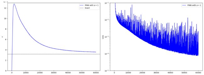
5.结果展示
训练过程,参数变化图如图3所示。可以清楚看到,在训练的早期,使用了自适应激活函数的PINN能够更快的下降并收敛到exact value。
训练过程中预测结果图如图4-6。