【机器学习】信用卡欺诈检测 （下采样、SMOTE过采样、集成学习、Pytorch）

2022.4.17 补充

视频：【参考：6-01 信用卡交易欺诈数据检测 _哔哩哔哩_bilibili】

【参考：机器学习/Kaggle/信用卡欺诈检测/Tommy/数据不平衡.ipynb · myaijarvis/AI - 码云 - 开源中国】

• 数据处理

【参考：机器学习/Kaggle/信用卡欺诈检测/Tommy/01 方案1 下采样.ipynb · myaijarvis/AI - 码云 - 开源中国】

• 下采样 集成学习

【参考：机器学习/Kaggle/信用卡欺诈检测/Tommy/02 版 SMOTE过采样&&下采样.ipynb · myaijarvis/AI - 码云 - 开源中国】

• SMOTE过采样 下采样 集成学习

【参考：机器学习/Kaggle/信用卡欺诈检测/Tommy/03 版 PyTorch深度学习.ipynb · myaijarvis/AI - 码云 - 开源中国】

• PyTorch深度学习 （效果非常好）

---

【参考：机器学习项目实战之信用卡欺诈检测（零基础，附数据及详细python代码）_西南交大-Liu_z的博客-CSDN博客】

【参考：实战六：kaggle实战之信用卡欺诈检测_超级圈的博客-CSDN博客】

【参考：【机器学习项目实战】很强！Kaggle竞赛案例+时间序列项目+Gensim中文词向量建模+MNIST手写数字识别+Python文本数据分析全套实战给大家安排！！_哔哩哔哩_bilibili p4-p13】

代码：【参考：机器学习/Kaggle/信用卡欺诈检测/信用卡欺诈检测.ipynb · myaijarvis/AI - 码云 - 开源中国】

分析目的

【参考：kaggle信用卡欺诈识别项目 - 知乎】
【参考：信用卡欺诈检测 | Kaggle】

利用大量数据，通过逻辑回归的算法，检验模型的效果，即模型识别出欺诈交易的有效性。从而能够在后续行为发生时，能够尽早识别，甚至是提前识别，带来商业价值。

评价指标

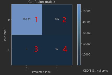
上面 0 正常 1 异常

查全率 56324/(56324+9) 1 / (1+3)
查准率 56324/(56324+537) 1 / (1+2)
精度 （56324+92）/ all (1+4) / (1+2+3+4)
误杀 537 右上角的 2
漏判 9 左下角 3

观察数据

import itertools

import numpy as np
import pandas as pd
import matplotlib.pyplot as plt

# 【参考：[信用卡欺诈检测数据集_唯一的阿金的博客-CSDN博客](https://blog.csdn.net/czjl6886/article/details/108073356)】
data = pd.read_csv('creditcard.csv')
data.head()

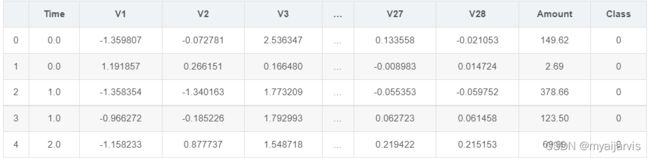
从数据的前五行中可以看出数据已经经过降维处理，这样的数据有好处也有坏处，好处就是我们不需要对数据再进行预处理，坏处就是数据具体代表的含义就不是很清楚了，这个案列中我们不再追究V1,V2….分别代表什么含义。

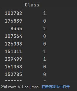
其中Amount的浮动范围很大，因此在稍后的过程中要进行归一化处理，Class代表分类标签，如果Class为0，代表这条交易是正常的交易，如果Class为1，代表这条交易确实存在欺诈行为。下面以柱状图的形式来对标签分类情况进行观察。

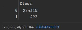
count_classes = pd.value_counts(data['Class'], sort=True)
count_classes

# 【参考：[[python] pandas plot画图命令总结_LandH的Blog的博客-CSDN博客](https://blog.csdn.net/u013084616/article/details/79064408)】
count_classes.plot(kind='bar', figsize=(10, 5), title='Frand class histogram')
plt.xlabel('Class')
plt.ylabel('Frequency')

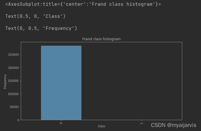
从图中可以看出标签为0的很多，而标签为1的却很少，说明样本的分布情况是非常不均衡的，所以在构建分类器的时候要特别注意一个误区，即使将结果全部预测为0也会出现很好的分类结果，这是在下文中需要着重考虑的一点。

数据处理

标准化操作

# 【参考：[sklearn.preprocessing.StandardScaler-scikit-learn中文社区](https://scikit-learn.org.cn/view/753.html)】
from sklearn.preprocessing import StandardScaler

stand = StandardScaler()  # 这是一个类,需要实例化
# fit_transform 拟合数据，然后对其进行转换。
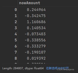
data['nowAmount'] = stand.fit_transform(
    data['Amount'].values.reshape(-1, 1))  # data['Amount']是Series类型，需要转化成numpy的ndarray
# reshape(-1,1) 转化为1列
# 【参考：[Series object has no attribute reshape解决方法_独自流浪的巨蟹的博客-CSDN博客](https://blog.csdn.net/weixin_41274723/article/details/106598281)】
data['nowAmount']

data['Amount'].shape

(284807,)

type(data['Amount'])

pandas.core.series.Series

data.Amount.values

array([149.62,   2.69, 378.66, ...,  67.88,  10.  , 217.  ])

type(data.Amount.values)

numpy.ndarray

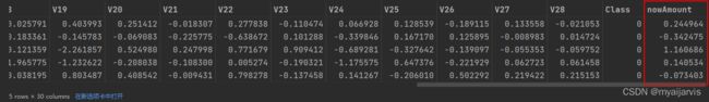
data = data.drop(['Time', 'Amount'], axis=1)  # 删除这两列 因为不需要
data.head()

下采样

要解决样本分布不均衡的问题，可以采用
**Undersample(下采样，即使样本数据变的一样少)**和
Oversample(过采样，即使样本数据变的一样多)。

下面代码采用下采样，即在class=0的标签中随机选取跟class=1一样多的样本数。

# 切分特征值和标签值
X = data.loc[:, data.columns != 'Class']  # 取除Class列以外的所有列
y = data.loc[:, data.columns == 'Class']  # 只取Class列

# fraud 欺诈 Class==1 / normal 正常 Class==0 / indices索引

number_records_fraud = len(data[data['Class'] == 1])  # 欺诈样本的数量 492

# 取欺诈样本的索引
fraud_indices = np.array(data[data['Class'] == 1].index)  # data['Class'] == 1 会返回一串 Ture False 字符串列表，再把这个当作索引
# 取正常样本的索引
normal_indices = data[data['Class'] == 0].index

# 下采样，使得两个样本同样少
#print(normal_indices)
#print(number_records_fraud)
# 随机生成正常样本的索引 / 在normal_indices中选number_records_fraud个 / 这里normal_indices远大于number_records_fraud / replace 所取样本是否能有重复值
random_normal_indices = np.random.choice(a=normal_indices, size=number_records_fraud, replace=False)
random_normal_indices = np.array(random_normal_indices)

# 将class=1和class=0 的选出来的索引值进行合并 此时这两个样本的数量是一样的
under_sample_indices = np.concatenate([fraud_indices, random_normal_indices])

under_sample_data = data.iloc[under_sample_indices, :]  # 取对应索引的数据

# 切分特征值和标签值
X_under_sample = under_sample_data.loc[:, under_sample_data.columns != 'Class']
y_under_sample = under_sample_data.loc[:, under_sample_data.columns == 'Class']

# Showing ratio
print("Percentage of normal transactions: ",
      len(under_sample_data[under_sample_data.Class == 0]) / len(under_sample_data))
print("Percentage of fraud transactions: ",
      len(under_sample_data[under_sample_data.Class == 1]) / len(under_sample_data))
print("Total number of transactions in resampled data: ", len(under_sample_data))

Percentage of normal transactions:  0.5
Percentage of fraud transactions:  0.5
Total number of transactions in resampled data:  984

数据切分

对数据集的训练是通过下采样的训练集，对数据的测试的是通过原始的数据集的测试集，下采样的测试集可能没有原始部分当中的一些特征，不能充分进行测试。

from sklearn.model_selection import train_test_split

# 原始样本用于测试
X_train, X_test, y_train, y_test = train_test_split(X, y, test_size=0.3, random_state=0)
#随机切分，random_state=0类似设置随机数种子，test_size就是测试集比例，我这里设置为0.3即0.7训练集，0.3测试集

print("原始样本训练集:", len(X_train))
print("原始样本测试集: ", len(X_test))
print("原始样本总数:", len(X_train) + len(X_test))

# 下采样样本用于训练
# 类型还是DataFrame
X_train_undersample, X_test_undersample, y_train_undersample, y_test_undersample = train_test_split(X_under_sample,y_under_sample,test_size=0.3,random_state=0)

print("下采样样本训练集: ", len(X_train_undersample))
print("下采样样本测试集: ", len(X_test_undersample))
print("下采样样本总数:", len(X_train_undersample) + len(X_test_undersample))

原始样本训练集: 199364
原始样本测试集:  85443
原始样本总数: 284807
下采样样本训练集:  688
下采样样本测试集:  296
下采样样本总数: 984

训练数据

交叉验证

使用逻辑回归模型构建分类器，通过k折交叉验证寻找最优惩罚参数

由于本文数据的特殊性，模型的评估的方法十分钟重要，通常采用的评价指标有准确率、召回率和F值（F-Measure）等。本文采用**recall（召回率）**作为评估标准。

具体举个例子介绍：假设我们在医院中有1000个病人，其中990个为正样本（正常），10个为负样本（癌症），我们的目的是找出其中的10个负样本，假如我们的模型将多有的1000个病人都预测为正样本，虽然精度有99%，但是并没有找到我们所要的10个负样本，所以这个模型是没用的，因为一个癌症病人都找不出来。而recall是对于想找的东西，找到了多少个，而不是所有样本的精度。

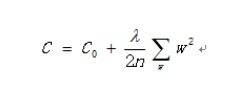
在构造权重参数的时候，为了防止过拟合的现象发生，要引入正则化惩罚项，使这些权重参数处于比较平滑的趋势，具体参数选择在代码中会给出解释。

from sklearn.linear_model import LogisticRegression  # 逻辑回归
# KFlod指做几倍的交叉验证，cross_val_score为交叉验证评估结果
from sklearn.model_selection import KFold, cross_val_score
# confusion_matrix 混淆矩阵 recall_score 召回率
from sklearn.metrics import confusion_matrix, recall_score, classification_report

import warnings

warnings.filterwarnings("ignore")

下面就是为了找到一个最合适的C值

# 参数类型为DataFrame
def print_KFold(X_train_data, y_train_data):
    # 【参考：[sklearn.model_selection.KFold-scikit-learn中文社区](https://scikit-learn.org.cn/view/636.html)】
    flod = KFold(n_splits=5, shuffle=False)
    #不同的惩罚参数C的参数集，因为不知道哪一种惩罚参数的力度好，通过验证集结果来选择
    c_param_range = [0.01, 0.1, 1, 10, 100]
    result = pd.DataFrame(index=[0, 1, 2, 3, 4], columns=['C_param', 'Mean recall score'])  # 建立一个DF以便后面记录数据
    result['C_param'] = c_param_range

    j = 0
    for c_param in c_param_range:
        print('-------------------------------------------')
        print('C parameter:', c_param)
        print('-------------------------------------------')

        recall_accs = []
        # split 返回 切分的训练集索引ndarray 切分的测试集索引ndarray
        for train_index, test_index in flod.split(X_train_data, y_train_data):
            # 【参考：[sklearn.linear_model.LogisticRegression-scikit-learn中文社区](https://scikit-learn.org.cn/view/378.html)】
            # C是惩罚力度，penalty是选择l1还是l2惩罚，solver可选参数:{‘liblinear’, ‘sag’, ‘saga’,‘newton-cg’, ‘lbfgs’}
            lr = LogisticRegression(penalty='l1', C=c_param, solver='liblinear')  # C 正则强度的倒数

            lr.fit(X_train_data.iloc[train_index, :], y=y_train_data.iloc[train_index, :])
            y_pred = lr.predict(X_train_data.iloc[test_index, :])
            # 【参考：[sklearn.metrics.recall_score-scikit-learn中文社区](https://scikit-learn.org.cn/view/499.html)】
            recall = recall_score(y_train_data.iloc[test_index, :], y_pred)

            recall_accs.append(recall)
            print("此次召回率:", recall)
        print('平均召回率:', np.mean(recall_accs))

        result.loc[j, 'Mean recall score'] = np.mean(recall_accs)
        j += 1
        print('平均召回率为:', np.mean(recall_accs))

    print(result)
    result['Mean recall score'] = result['Mean recall score'].astype('float64')
    best_c = result.loc[result['Mean recall score'].idxmax()]['C_param']
    print("最好的参数C:", best_c)
    return best_c

best_c = print_KFold(X_train_undersample, y_train_undersample)

-------------------------------------------
C parameter: 0.01
-------------------------------------------
此次召回率: 0.9726027397260274
此次召回率: 0.9452054794520548
此次召回率: 1.0
此次召回率: 0.972972972972973
此次召回率: 0.9848484848484849
平均召回率: 0.9751259353999082
平均召回率为: 0.9751259353999082
-------------------------------------------
C parameter: 0.1
-------------------------------------------
此次召回率: 0.8356164383561644
此次召回率: 0.863013698630137
此次召回率: 0.9491525423728814
此次召回率: 0.918918918918919
此次召回率: 0.8939393939393939
平均召回率: 0.8921281984434991
平均召回率为: 0.8921281984434991
-------------------------------------------
C parameter: 1
-------------------------------------------
此次召回率: 0.8493150684931506
此次召回率: 0.8767123287671232
此次召回率: 0.9661016949152542
此次召回率: 0.9459459459459459
此次召回率: 0.9090909090909091
平均召回率: 0.9094331894424765
平均召回率为: 0.9094331894424765
-------------------------------------------
C parameter: 10
-------------------------------------------
此次召回率: 0.863013698630137
此次召回率: 0.8767123287671232
此次召回率: 0.9661016949152542
此次召回率: 0.9459459459459459
此次召回率: 0.9242424242424242
平均召回率: 0.9152032185001768
平均召回率为: 0.9152032185001768
-------------------------------------------
C parameter: 100
-------------------------------------------
此次召回率: 0.863013698630137
此次召回率: 0.8767123287671232
此次召回率: 0.9661016949152542
此次召回率: 0.9459459459459459
此次召回率: 0.9242424242424242
平均召回率: 0.9152032185001768
平均召回率为: 0.9152032185001768
   C_param Mean recall score
0     0.01          0.975126
1     0.10          0.892128
2     1.00          0.909433
3    10.00          0.915203
4   100.00          0.915203
最好的参数C: 0.01

type(X_train_undersample)

pandas.core.frame.DataFrame

y_train_undersample.shape

(688, 1)

X_train_undersample.shape

(688, 29)

混淆矩阵

from sklearn.metrics import precision_score, recall_score, f1_score

lr = LogisticRegression(penalty='l1', C=best_c, solver='liblinear')

# X:(n_samples, n_features) y:(n_samples,)
lr.fit(X_train_undersample, y_train_undersample)
y_pred_undersample = lr.predict(X_train_undersample)

matrix = confusion_matrix(y_train_undersample, y_pred_undersample)

print("混淆矩阵:\n", matrix)
print("精度:", precision_score(y_train_undersample, y_pred_undersample))
print("召回率:", recall_score(y_train_undersample, y_pred_undersample))
print("f1分数:", f1_score(y_train_undersample, y_pred_undersample))

LogisticRegression(C=0.01, penalty='l1', solver='liblinear')
混淆矩阵:
 [[302  41]
 [ 20 325]]
精度: 0.8879781420765027
召回率: 0.9420289855072463
f1分数: 0.9142053445850914

使用下采样数据训练与测试

import itertools


# cm:confusion_matrix 矩阵数据（2，2） / classes 分类 后面会传[0,1]
def plot_confusion_matrix(cm, classes,title='Confusion matrix'):
    #cm为数据，interpolation='nearest'使用最近邻插值，cmap颜色图谱（colormap), 默认绘制为RGB(A)颜色空间
    plt.imshow(X=cm, cmap=plt.cm.Blues, interpolation='nearest')
    plt.title(title)
    plt.colorbar()  # 设置颜色条
    tick_marks = np.arange(len(classes))
    # 画刻度 xticks(刻度下标，刻度标签)
    plt.xticks(ticks=tick_marks, labels=classes, rotation=0)
    plt.yticks(ticks=tick_marks, labels=classes, rotation=0)
    thresh = cm.max() / 2 # .max() 取矩阵中最大的数据
    #text()命令可以在任意的位置添加文字
    # 【参考：[python画图时给图中的点加标签之plt.text_帅帅de三叔的博客-CSDN博客](https://blog.csdn.net/zengbowengood/article/details/104324293)】
    for i, j in itertools.product(range(cm.shape[0]), range(cm.shape[1])): # i，j：0，1
        plt.text(j, i, # 坐标
                 s=cm[i, j], # 标签的符号 这里是数字
                 horizontalalignment='center',
                 color='white' if cm[i, j] > thresh else 'black') # 颜色

    #自动紧凑布局
    plt.tight_layout()
    plt.ylabel('True label')
    plt.xlabel('Predicted label')

lr = LogisticRegression(C = best_c, penalty = 'l1',solver='liblinear')
lr.fit(X_train_undersample,y_train_undersample)
y_pred_undersample = lr.predict(X_test_undersample)
#计算混淆矩阵
# 【参考：[sklearn.metrics.confusion_matrix-scikit-learn中文社区](https://scikit-learn.org.cn/view/485.html)】
cnf_matrix = confusion_matrix(y_test_undersample,y_pred_undersample)
#输出精度为小数点后两位
np.set_printoptions(precision=2)
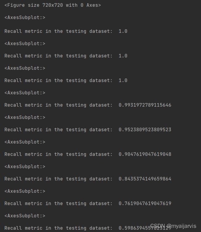
print("Recall metric in the testing dataset: ", cnf_matrix[1,1]/(cnf_matrix[1,0]+cnf_matrix[1,1]))
#画出非标准化的混淆矩阵
class_names = [0,1]
plt.figure()
plot_confusion_matrix(cnf_matrix,classes=class_names)
plt.show()

Recall metric in the testing dataset:  0.9523809523809523

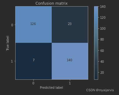
cnf_matrix

array([[126,  23],
       [  7, 140]], dtype=int64)

cnf_matrix.max()

140

使用下采样数据训练，使用原始数据测试

lr = LogisticRegression(C = best_c, penalty = 'l1',solver='liblinear')
lr.fit(X_train_undersample,y_train_undersample)
y_pred = lr.predict(X_test) # 注意，这里使用的是原始数据
#计算混淆矩阵
# 【参考：[sklearn.metrics.confusion_matrix-scikit-learn中文社区](https://scikit-learn.org.cn/view/485.html)】
cnf_matrix = confusion_matrix(y_test,y_pred)
#输出精度为小数点后两位
np.set_printoptions(precision=2)
print("Recall metric in the testing dataset: ", cnf_matrix[1,1]/(cnf_matrix[1,0]+cnf_matrix[1,1]))
#画出非标准化的混淆矩阵
class_names = [0,1]
plt.figure()
plot_confusion_matrix(cnf_matrix,classes=class_names)
plt.show()

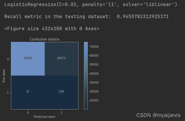
小结：虽然recall值可达到94.6%，但是其中有10672个数据本来不存在欺诈行为，却检测成了欺诈行为，这还是一个挺头疼的问题。 右上角是被误杀的

如果大家对结果表示怀疑，想着如果用原始数据来训练是否会有更好地效果呢？那么我们不妨用原始数据训练一次试试，代码前面已经写了，只需调用即可。

使用原始数据进行训练与测试

先使用使用原始数据训练找到最合适的C

best_c = print_KFold(X_train,y_train)

-------------------------------------------
C parameter: 0.01
-------------------------------------------
此次召回率: 0.4925373134328358
此次召回率: 0.6027397260273972
此次召回率: 0.6833333333333333
此次召回率: 0.5692307692307692
此次召回率: 0.45
平均召回率: 0.5595682284048672
平均召回率为: 0.5595682284048672
-------------------------------------------
C parameter: 0.1
-------------------------------------------
此次召回率: 0.5671641791044776
此次召回率: 0.6164383561643836
此次召回率: 0.6833333333333333
此次召回率: 0.5846153846153846
此次召回率: 0.525
平均召回率: 0.5953102506435158
平均召回率为: 0.5953102506435158
-------------------------------------------
C parameter: 1
-------------------------------------------
此次召回率: 0.5522388059701493
此次召回率: 0.6164383561643836
此次召回率: 0.7166666666666667
此次召回率: 0.6153846153846154
此次召回率: 0.5625
平均召回率: 0.612645688837163
平均召回率为: 0.612645688837163
-------------------------------------------
C parameter: 10
-------------------------------------------
此次召回率: 0.5522388059701493
此次召回率: 0.6164383561643836
此次召回率: 0.7333333333333333
此次召回率: 0.6153846153846154
此次召回率: 0.575
平均召回率: 0.6184790221704963
平均召回率为: 0.6184790221704963
-------------------------------------------
C parameter: 100
-------------------------------------------
此次召回率: 0.5522388059701493
此次召回率: 0.6164383561643836
此次召回率: 0.7333333333333333
此次召回率: 0.6153846153846154
此次召回率: 0.575
平均召回率: 0.6184790221704963
平均召回率为: 0.6184790221704963
   C_param Mean recall score
0     0.01          0.559568
1     0.10           0.59531
2     1.00          0.612646
3    10.00          0.618479
4   100.00          0.618479
最好的参数C: 10.0

再使用原始数据进行训练与测试

lr = LogisticRegression(C = best_c, penalty = 'l1',solver='liblinear')
lr.fit(X_train,y_train) # 注意，这里使用的是原始数据
y_pred = lr.predict(X_test) # 注意，这里使用的是原始数据
#计算混淆矩阵
# 【参考：[sklearn.metrics.confusion_matrix-scikit-learn中文社区](https://scikit-learn.org.cn/view/485.html)】
cnf_matrix = confusion_matrix(y_test,y_pred)
#输出精度为小数点后两位
np.set_printoptions(precision=2)
print("Recall metric in the testing dataset: ", cnf_matrix[1,1]/(cnf_matrix[1,0]+cnf_matrix[1,1]))
#画出非标准化的混淆矩阵
class_names = [0,1]
plt.figure()
plot_confusion_matrix(cnf_matrix,classes=class_names)
plt.show()

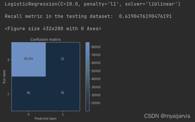
从图中可以看出虽然对正常样本的检测效果很好，但是在欺诈样本中的检测确实很不理想，这个分类器的精度是比较高的，但是它的recall值确实比较低的。

使用下采样数据训练与测试（不同的阈值）

逻辑回归的sigmoid函数中，一般来说阈值为0.5（即大于0.5的判为1）
但是也可以自定义不同的阈值，看其是否对最终的结果有影响

这里best_c是0.01

lr = LogisticRegression(C = 0.01, penalty = 'l1',solver='liblinear')
lr.fit(X_train_undersample,y_train_undersample)
y_pred_undersample_proba = lr.predict_proba(X_test_undersample) # predict_proba 输出概率值

type(y_pred_undersample_proba)
y_pred_undersample_proba.shape 

numpy.ndarray
(296, 2)

y_pred_undersample_proba

array([[5.22e-01, 4.78e-01],
       [3.92e-01, 6.08e-01],
       [2.20e-03, 9.98e-01],
       [6.01e-01, 3.99e-01],
       [5.81e-01, 4.19e-01],
      
       [6.19e-01, 3.81e-01],
       [4.05e-01, 5.95e-01],
       [4.21e-01, 5.79e-01],
       [6.15e-01, 3.85e-01]])

y_pred_undersample_proba[:,1] > 0.6

array([False,  True,  True, False, False,  True,  True, False, False,
       False,  True, False,  True,  True, False,  True, False, False,
        True,  True,  True, False,  True, False,  True, False,  True,
       
        True, False, False, False,  True,  True,  True,  True, False,
        True,  True, False,  True, False, False, False, False])

y_test_undersample # 0,1组成的ndarray

thresholds=[0.1,0.2,0.3,0.4,0.5,0.6,0.7,0.8,0.9] # 阈值的大小

plt.figure(figsize=(10,10)) # 设置画布大小 1000*1000

j=1
for i in thresholds:
    y_test_predict_high_recall=y_pred_undersample_proba[:,1] > i # 大于阈值的样本

    plt.subplot(3,3,j) # 设置子图位置
    j+=1
    #计算混淆矩阵
    cnf_matrix = confusion_matrix(y_test_undersample,y_test_predict_high_recall) # 两个数据进行对比
    #输出精度为小数点后两位
    np.set_printoptions(precision=2)
    print("Recall metric in the testing dataset: ", cnf_matrix[1,1]/(cnf_matrix[1,0]+cnf_matrix[1,1]))
    #画出非标准化的混淆矩阵
    class_names = [0,1]

    plot_confusion_matrix(cnf_matrix,classes=class_names,title='Threshold >= %s'%i)

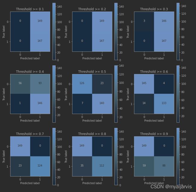
小结：从以上的实验可以看出，虽然在阈值设置较小的时候，recall值可以达到1，但是此时模型的精度却太低，此模型就有一种宁可错杀一千，也不可放过一百的感觉。。。当阈值变大时，模型的精度会逐渐上升，recall值稍稍减少，但阈值过大时，模型的精度也会适当减少，而recall值这回大大减小。

SMOTE 过采样

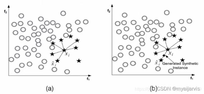
在使用过采样之前，首先介绍下SMOTE算法，其基本原理为：
1、对于少数类中的每一个样本x，以欧式距离计算它到少数类样本集中所有样本的距离，得到其k近邻
2、根据样本不平衡比例设置一个采样比例以确定采样倍率N，对于每一个少类样本x，从其k近邻中随机选择若干个样本，假设选择的近邻为xn
3、对于每一个随机选出的近邻xn，分别与原样本按照如下的公式构建新的样本。


SMOTEENN

from imblearn.combine import SMOTEENN 
# 结合过采样和下采样
#Combine over- and under-sampling using SMOTE and Edited Nearest Neighbours.

smote_enn=SMOTEENN(random_state=0)
x,y=smote_enn.fit_resample(x,y)

构造过采样的数据

import pandas as pd
from imblearn.over_sampling import SMOTE
from sklearn.metrics import confusion_matrix
from sklearn.model_selection import train_test_split

credit_cards=pd.read_csv('creditcard.csv')
columns=credit_cards.columns

# 为了获得特征列，移除最后一列标签列 为什么要这样？
features_columns=columns.delete(len(columns)-1)
features=credit_cards[features_columns]
labels=credit_cards['Class']

features_train, features_test, labels_train, labels_test = train_test_split(features,
                                                                            labels,
                                                                            test_size=0.2,
                                                                            random_state=0)

oversampler=SMOTE(random_state=0)
os_features,os_labels=oversampler.fit_sample(features_train,labels_train) # 只需要对训练集过采样增加数据来训练，测试集不需要

len(os_labels[os_labels==1]) # 欺诈样本和正常样本现在是一样多的了

227454

K折交叉验证得到最好的惩罚参数C

os_features = pd.DataFrame(os_features)
os_labels = pd.DataFrame(os_labels)
best_c = print_KFold(os_features,os_labels)

过程省略
最好的参数C: 10.0

逻辑回归计算混淆矩阵以及召回率

使用过采样数据进行训练，使用原始数据进行测试

lr = LogisticRegression(C = best_c, penalty = 'l1',solver='liblinear')
lr.fit(os_features,os_labels)
y_pred = lr.predict(features_test)
#计算混淆矩阵
# 【参考：[sklearn.metrics.confusion_matrix-scikit-learn中文社区](https://scikit-learn.org.cn/view/485.html)】
cnf_matrix = confusion_matrix(labels_test,y_pred)
#输出精度为小数点后两位
np.set_printoptions(precision=2)
print("Recall metric in the testing dataset: ", cnf_matrix[1,1]/(cnf_matrix[1,0]+cnf_matrix[1,1]))
#画出非标准化的混淆矩阵
class_names = [0,1]
plt.figure()
plot_confusion_matrix(cnf_matrix,classes=class_names)
plt.show()

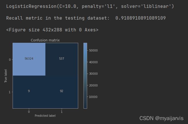
小结：虽然过采样的recall值比下采样稍小，但是它的精度却大大提高了，即减少了误杀的数量，所以在出现数据不均衡的情况下，较经常使用的是生成数据而不是减少数据，但是数据一旦多起来，运行时间也变长了。

查全率 56324/(56324+9)
查准率 56324/(56324+537)
精度 （56324+92）/ all

End

可以参考一下大佬的思路和代码
https://www.kaggle.com/datasets/mlg-ulb/creditcardfraud/code?datasetId=310&sortBy=voteCount&language=Python