精通特征工程 —— 2.简单得数字奇特技巧

精通特征工程pdf：链接：https://pan.baidu.com/s/11AFe7LgjYnf56XcpI_wNKw 提取码：fvzo
参考黄博代码实现：https://github.com/fengdu78/Data-Science-Notes/tree/master/9.feature-engineering

1.二值化

# Echo Nest 品味画像数据集的统计
# 使 Million Song 数据集中听歌计数二进制化
import pandas as pd
f = open(r'data/train_triplets.txt')
listen_count = pd.read_csv(f, header=None, delimiter='\t')
listen_count[2] = 1

listen_count.head()

	0	1	2
0	b80344d063b5ccb3212f76538f3d9e43d87dca9e	SOAKIMP12A8C130995	1
1	b80344d063b5ccb3212f76538f3d9e43d87dca9e	SOAPDEY12A81C210A9	1
2	b80344d063b5ccb3212f76538f3d9e43d87dca9e	SOBBMDR12A8C13253B	1
3	b80344d063b5ccb3212f76538f3d9e43d87dca9e	SOBFNSP12AF72A0E22	1
4	b80344d063b5ccb3212f76538f3d9e43d87dca9e	SOBFOVM12A58A7D494	1

2.区间量化（分箱）

# Yelp 数据集中的商家点评数量可视化 
import pandas as pd
import json
# 加载商家数据
biz_file = open('data/yelp_academic_dataset_business.json')
biz_df = pd.DataFrame([json.loads(x) for x in biz_file.readlines()])
biz_file.close()

biz_df.head()

	business_id	categories	city	full_address	latitude	longitude	name	neighborhoods	open	review_count	stars	state	type
0	rncjoVoEFUJGCUoC1JgnUA	[Accountants, Professional Services, Tax Servi...	Peoria	8466 W Peoria Ave\nSte 6\nPeoria, AZ 85345	33.581867	-112.241596	Peoria Income Tax Service	[]	True	3	5.0	AZ	business
1	0FNFSzCFP_rGUoJx8W7tJg	[Sporting Goods, Bikes, Shopping]	Phoenix	2149 W Wood Dr\nPhoenix, AZ 85029	33.604054	-112.105933	Bike Doctor	[]	True	5	5.0	AZ	business
2	3f_lyB6vFK48ukH6ScvLHg	[]	Phoenix	1134 N Central Ave\nPhoenix, AZ 85004	33.460526	-112.073933	Valley Permaculture Alliance	[]	True	4	5.0	AZ	business
3	usAsSV36QmUej8--yvN-dg	[Food, Grocery]	Phoenix	845 W Southern Ave\nPhoenix, AZ 85041	33.392210	-112.085377	Food City	[]	True	5	3.5	AZ	business
4	PzOqRohWw7F7YEPBz6AubA	[Food, Bagels, Delis, Restaurants]	Glendale Az	6520 W Happy Valley Rd\nSte 101\nGlendale Az, ...	33.712797	-112.200264	Hot Bagels & Deli	[]	True	14	3.5	AZ	business

# 绘制点评数量直方图
import matplotlib.pyplot as plt
import seaborn as sns
%matplotlib inline

sns.set_style('whitegrid')
fig, ax = plt.subplots()
biz_df['review_count'].hist(ax=ax, bins=100)
ax.set_yscale('log')
ax.tick_params(labelsize=14)
ax.set_xlabel('Review Count', fontsize=14)
ax.set_ylabel('Occurrence', fontsize=14)

Text(0, 0.5, 'Occurrence')

# 通过固定宽度分箱对计数值进行区间量化 
import numpy as np

# 生成20个随机整数，均匀分布在0-99之间
small_counts = np.random.randint(0, 100, 20)
small_counts

array([13, 48, 98, 20, 58, 21, 92, 19, 48, 31, 46, 86, 23, 45, 65, 60, 66,
       42, 20,  9])

# 通过出发映射到间隔均匀的分箱中，每个分箱取值范围0-9
np.floor_divide(small_counts, 10)

array([1, 4, 9, 2, 5, 2, 9, 1, 4, 3, 4, 8, 2, 4, 6, 6, 6, 4, 2, 0], dtype=int32)

# 横跨若干数量级的计数值数组
large_counts =  [296, 8286, 64011, 80, 3, 725, 867, 2215, 7689, 11495, 91897, 
                 44, 28, 7971, 926, 122, 22222] 
# 通过对数函数映射到指数宽度分箱
np.floor(np.log10(large_counts))

array([ 2.,  3.,  4.,  1.,  0.,  2.,  2.,  3.,  3.,  4.,  4.,  1.,  1.,
        3.,  2.,  2.,  4.])

# 计算 Yelp 商家点评数量的十分位数
deciles = biz_df['review_count'].quantile([.1, .2, .3, .4, .5, .6, .7, .8, .9])
deciles

0.1     3.0
0.2     3.0
0.3     4.0
0.4     5.0
0.5     6.0
0.6     8.0
0.7    12.0
0.8    23.0
0.9    50.0
Name: review_count, dtype: float64

# 在直方图上画出十分位数
sns.set_style('whitegrid')
fig, ax = plt.subplots()
biz_df['review_count'].hist(ax=ax, bins=100)
for pos in deciles:
    handle = plt.axvline(pos, color='r')
ax.legend([handle], ['deciles'], fontsize=14)
ax.set_yscale('log')
ax.set_xscale('log')
ax.tick_params(labelsize=14)
ax.set_xlabel('Review Count', fontsize=14)
ax.set_ylabel('Occurence', fontsize=14)

Text(0, 0.5, 'Occurence')

# 通过分位数对计数值进行分箱 
# 使用large_counts
pd.qcut(large_counts, 4, labels=False)  # 将数据映射为所需的分位数值

array([1, 2, 3, 0, 0, 1, 1, 2, 2, 3, 3, 0, 0, 2, 1, 0, 3], dtype=int64)

# 计算实际的分位数值
large_counts_series = pd.Series(large_counts)
large_counts_series.quantile([0.25, 0.5, 0.75])

0.25     122.0
0.50     926.0
0.75    8286.0
dtype: float64

3.对数变换

# 对数函数可以将大数值的范围压缩，对小数值的范围进行扩展
# 对数变换前后的点评数量分布可视化
fig, (ax1, ax2) = plt.subplots(2,1)
fig.tight_layout(pad=0, w_pad=4.0, h_pad=4.0)
biz_df['review_count'].hist(ax=ax1, bins=100)
ax1.tick_params(labelsize=14)
ax1.set_xlabel('review_count', fontsize=14)
ax1.set_ylabel('Occurrence', fontsize=14)
biz_df['log_review_count'] = np.log(biz_df['review_count'] + 1)
biz_df['log_review_count'].hist(ax=ax2, bins=100)
ax2.tick_params(labelsize=14)
ax2.set_xlabel('log10(review_count))', fontsize=14)
ax2.set_ylabel('Occurrence', fontsize=14)

Text(23.625, 0.5, 'Occurrence')

在线新闻流行度数据集的统计信息
目标是使用这些特征来预测文章的流行度，流行度用社交媒体上的分享数表示,研究一个特征——文章中的单词个数

df = pd.read_csv('data/OnlineNewsPopularity.csv', delimiter=', ')
df.head()

C:\Users\S2\Anaconda3\lib\site-packages\ipykernel\__main__.py:1: ParserWarning: Falling back to the 'python' engine because the 'c' engine does not support regex separators (separators > 1 char and different from '\s+' are interpreted as regex); you can avoid this warning by specifying engine='python'.
  if __name__ == '__main__':

	url	timedelta	n_tokens_title	n_tokens_content	n_unique_tokens	n_non_stop_words	n_non_stop_unique_tokens	num_hrefs	num_self_hrefs	num_imgs	...	min_positive_polarity	max_positive_polarity	avg_negative_polarity	min_negative_polarity	max_negative_polarity	title_subjectivity	title_sentiment_polarity	abs_title_subjectivity	abs_title_sentiment_polarity	shares
0	http://mashable.com/2013/01/07/amazon-instant-...	731.0	12.0	219.0	0.663594	1.0	0.815385	4.0	2.0	1.0	...	0.100000	0.7	-0.350000	-0.600	-0.200000	0.500000	-0.187500	0.000000	0.187500	593
1	http://mashable.com/2013/01/07/ap-samsung-spon...	731.0	9.0	255.0	0.604743	1.0	0.791946	3.0	1.0	1.0	...	0.033333	0.7	-0.118750	-0.125	-0.100000	0.000000	0.000000	0.500000	0.000000	711
2	http://mashable.com/2013/01/07/apple-40-billio...	731.0	9.0	211.0	0.575130	1.0	0.663866	3.0	1.0	1.0	...	0.100000	1.0	-0.466667	-0.800	-0.133333	0.000000	0.000000	0.500000	0.000000	1500
3	http://mashable.com/2013/01/07/astronaut-notre...	731.0	9.0	531.0	0.503788	1.0	0.665635	9.0	0.0	1.0	...	0.136364	0.8	-0.369697	-0.600	-0.166667	0.000000	0.000000	0.500000	0.000000	1200
4	http://mashable.com/2013/01/07/att-u-verse-apps/	731.0	13.0	1072.0	0.415646	1.0	0.540890	19.0	19.0	20.0	...	0.033333	1.0	-0.220192	-0.500	-0.050000	0.454545	0.136364	0.045455	0.136364	505

5 rows × 61 columns

df['log_n_tokens_content'] = np.log10(df['n_tokens_content'] + 1)

# 新闻文章流行度分布的可视化，使用对数变换和不使用对数变换 
fig, (ax1, ax2) = plt.subplots(2, 1)
df['n_tokens_content'].hist(ax=ax1, bins=100)
ax1.tick_params(labelsize=14)
ax1.set_xlabel('Number of Words in Article', fontsize=14)
ax1.set_ylabel('Number of Article', fontsize=14)

df['log_n_tokens_content'].hist(ax=ax2, bins=100)
ax1.tick_params(labelsize=14)
ax1.set_xlabel('Number of Words in Article', fontsize=14)
ax1.set_ylabel('Number of Article', fontsize=14)

Text(0, 0.5, 'Number of Article')

# 使用对数变换后的 Yelp 点评数量预测商家的平均评分 
from sklearn import linear_model
from sklearn.model_selection import cross_val_score

# 使用前面加载的yelp点评数据，计算yelp点评数量的对数变换值
# 注意：为原始点评数量加1，以免当点评数量为0时，对数运算结果得到负无穷大
biz_df['log_review_count'] = np.log10(biz_df['review_count'] + 1)

# 使用经过对数变换和未经过对数变换的review_count特征，训练线性回归模型预测
# 一个商家的平均星级评分，比较两种模型的10折交叉验证得分
m_orig = linear_model.LinearRegression()
scores_orig = cross_val_score(m_orig, biz_df[['review_count']], 
                             biz_df['stars'], cv=10)

m_log = linear_model.LinearRegression()
scores_log = cross_val_score(m_log, biz_df[['log_review_count']], 
                             biz_df['stars'], cv=10)

print("R-squared score without log transform: %0.5f (+/- %0.5f)" %
      (scores_orig.mean(), scores_orig.std() * 2))
print("R-squared score with log transform: %0.5f (+/- %0.5f)" %
      (scores_log.mean(), scores_log.std() * 2))

R-squared score without log transform: 0.00215 (+/- 0.00329)
R-squared score with log transform: 0.00136 (+/- 0.00328)

# 使用在线新闻流行度数据集中经对数变换后的单词个数预测文章流行度 
# 加载数据集
df = pd.read_csv('data/OnlineNewsPopularity.csv', delimiter=', ')
# 对n_tokens_content特征进行对数变换，特征表示新闻文章中的单词
df['log_n_tokens_content'] = np.log10(df['n_tokens_content'] + 1)

# 训练两个线性回归模型来预测文章分享数（初始特征，对数变换后特征）
m_orig = linear_model.LinearRegression()
scores_orig = cross_val_score(
    m_orig, df[['n_tokens_content']], df['shares'], cv=10)
m_log = linear_model.LinearRegression()
scores_log = cross_val_score(
    m_log, df[['log_n_tokens_content']], df['shares'], cv=10)

print("R-squared score without log transform: %0.5f (+/- %0.5f)" %
      (scores_orig.mean(), scores_orig.std() * 2))
print("R-squared score with log transform: %0.5f (+/- %0.5f)" %
      (scores_log.mean(), scores_log.std() * 2))

C:\Users\S2\Anaconda3\lib\site-packages\ipykernel\__main__.py:3: ParserWarning: Falling back to the 'python' engine because the 'c' engine does not support regex separators (separators > 1 char and different from '\s+' are interpreted as regex); you can avoid this warning by specifying engine='python'.
  app.launch_new_instance()


R-squared score without log transform: -0.00242 (+/- 0.00509)
R-squared score with log transform: -0.00114 (+/- 0.00418)

# 可视化新闻流程度预测问题中输入输出相关性
fig2, (ax1, ax2) = plt.subplots(2, 1,figsize=(10, 4))
fig.tight_layout(pad=0.4, w_pad=4.0, h_pad=6.0)
ax1.scatter(df['n_tokens_content'], df['shares'])
ax1.tick_params(labelsize=14)
ax1.set_xlabel('Number of Words in Article', fontsize=14)
ax1.set_ylabel('Number of Shares', fontsize=14)

ax2.scatter(df['log_n_tokens_content'], df['shares'])
ax2.tick_params(labelsize=14)
ax2.set_xlabel('Log of the Number of Words in Article', fontsize=14)
ax2.set_ylabel('Number of Shares', fontsize=14)

Text(0, 0.5, 'Number of Shares')

# 对 Yelp 商家点评数量的 Box-Cox 变换 
from scipy import stats
# 假设bie_df包含yelp商家点评数据，Box_Cox变换假定输入数据都是正的，
# 检查数据的最小值已确定满足假定
biz_df['review_count'].min()

3

# 设置输入参数lmbda为0，使用对数变换
rc_log = stats.boxcox(biz_df['review_count'], lmbda=0)
# scipy在实现box-cox转换时，会找出使得输出最接近与正态分布的lmbda参数
rc_bc, bc_params = stats.boxcox(biz_df['review_count'])
bc_params

-0.5631160899391674

4.特征缩放归一化

如果模型对输入特征的尺度很敏感，就需要进行特征缩放

min-max缩放
$$\tilde{x}=\frac{x-\min (x)}{\max (x)-\min (x)}$$

标准化（方差缩放）
$$\tilde{x}=\frac{x-\mathrm{mean}(x)}{\mathrm{sqrt}(\mathrm{var}(x))}$$

L2归一化
$$x=\frac{x}{\Vert x{\Vert }_2}$$

# 特征缩放实例
import sklearn.preprocessing as preproc

# 加载在线新闻流行度数据
df['n_tokens_content'].as_matrix()

array([ 219.,  255.,  211., ...,  442.,  682.,  157.])

# min-max缩放
df['minmax'] = preproc.minmax_scale(df[['n_tokens_content']])
df['minmax'].as_matrix()

array([ 0.02584376,  0.03009205,  0.02489969, ...,  0.05215955,
        0.08048147,  0.01852726])

# 标准化
df['standardized'] = preproc.StandardScaler().fit_transform(df[['n_tokens_content']])
df['standardized'].as_matrix()

array([-0.69521045, -0.61879381, -0.71219192, ..., -0.2218518 ,
        0.28759248, -0.82681689])

# L2 归一化
df['l2_normalized'] = preproc.normalize(df[['n_tokens_content']], axis=0)
df['l2_normalized'].as_matrix()

array([ 0.00152439,  0.00177498,  0.00146871, ...,  0.00307663,
        0.0047472 ,  0.00109283])

# 绘制原始数据和缩放后数据的直方图
fig, (ax1, ax2, ax3, ax4) = plt.subplots(4, 1)
fig.tight_layout()

df['n_tokens_content'].hist(ax=ax1, bins=100)
ax1.tick_params(labelsize=14)
ax1.set_xlabel('Article word count', fontsize=14)
ax1.set_ylabel('Number of articles', fontsize=14)

df['minmax'].hist(ax=ax2, bins=100)
ax2.tick_params(labelsize=14)
ax2.set_xlabel('min-max word count', fontsize=14)
ax2.set_ylabel('Number of articles', fontsize=14)

df['standardized'].hist(ax=ax3, bins=100)
ax3.tick_params(labelsize=14)
ax3.set_xlabel('standardized word count', fontsize=14)
ax3.set_ylabel('Number of articles', fontsize=14)

df['l2_normalized'].hist(ax=ax4, bins=100)
ax4.tick_params(labelsize=14)
ax4.set_xlabel('l2_normalized word count', fontsize=14)
ax4.set_ylabel('Number of articles', fontsize=14)

Text(29.125, 0.5, 'Number of articles')

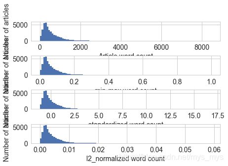
只有x轴尺度发生了变化，特征缩放后的分布形状不变

5.交互特征

# 预测中的交互特征实例
from sklearn import linear_model
from sklearn.model_selection import train_test_split
import sklearn.preprocessing as preproc

# df 包含UCI在线新闻流行度数据集
df.columns

Index(['url', 'timedelta', 'n_tokens_title', 'n_tokens_content',
       'n_unique_tokens', 'n_non_stop_words', 'n_non_stop_unique_tokens',
       'num_hrefs', 'num_self_hrefs', 'num_imgs', 'num_videos',
       'average_token_length', 'num_keywords', 'data_channel_is_lifestyle',
       'data_channel_is_entertainment', 'data_channel_is_bus',
       'data_channel_is_socmed', 'data_channel_is_tech',
       'data_channel_is_world', 'kw_min_min', 'kw_max_min', 'kw_avg_min',
       'kw_min_max', 'kw_max_max', 'kw_avg_max', 'kw_min_avg', 'kw_max_avg',
       'kw_avg_avg', 'self_reference_min_shares', 'self_reference_max_shares',
       'self_reference_avg_sharess', 'weekday_is_monday', 'weekday_is_tuesday',
       'weekday_is_wednesday', 'weekday_is_thursday', 'weekday_is_friday',
       'weekday_is_saturday', 'weekday_is_sunday', 'is_weekend', 'LDA_00',
       'LDA_01', 'LDA_02', 'LDA_03', 'LDA_04', 'global_subjectivity',
       'global_sentiment_polarity', 'global_rate_positive_words',
       'global_rate_negative_words', 'rate_positive_words',
       'rate_negative_words', 'avg_positive_polarity', 'min_positive_polarity',
       'max_positive_polarity', 'avg_negative_polarity',
       'min_negative_polarity', 'max_negative_polarity', 'title_subjectivity',
       'title_sentiment_polarity', 'abs_title_subjectivity',
       'abs_title_sentiment_polarity', 'shares', 'log_n_tokens_content',
       'minmax', 'standardized', 'l2_normalized'],
      dtype='object')

# 选择与内容有关的特征作为模型单一特征，忽略衍生特征
features = ['n_tokens_title', 'n_tokens_content',
            'n_unique_tokens', 'n_non_stop_words', 'n_non_stop_unique_tokens',
            'num_hrefs', 'num_self_hrefs', 'num_imgs', 'num_videos',
            'average_token_length', 'num_keywords', 'data_channel_is_lifestyle',
            'data_channel_is_entertainment', 'data_channel_is_bus',
            'data_channel_is_socmed', 'data_channel_is_tech',
            'data_channel_is_world']
X = df[features]
y = df['shares']

# 创建交互特征对，跳过固定偏移项
X2 = preproc.PolynomialFeatures(include_bias=False).fit_transform(X)
X2.shape

(39644, 170)

# 为两个特征集创建训练集和测试集
X1_train, X1_test, X2_train, X2_test, y_train, y_test = train_test_split(X, X2, y, test_size=0.3, random_state=123)

def evaluate_feature(X_train, X_test, y_train, y_test):
    model = linear_model.LinearRegression().fit(X_train, y_train)
    r_score = model.score(X_test, y_test)
    return (model, r_score)

# 在两个特征集上训练模型并比较R方分数
(m1, r1) = evaluate_feature(X1_train, X1_test, y_train, y_test)
(m2, r2) = evaluate_feature(X2_train, X2_test, y_train, y_test)
print("R-squared score with singleton features: %0.5f" % r1)
print("R-squared score with pairwise features: %0.10f" % r2)

R-squared score with singleton features: 0.00924
R-squared score with pairwise features: 0.0113280904

6.特征选择

• 过滤：对特征进行预处理
• 打包方法:对某特征提供的方法
• 嵌入式方法：模型训练