CS231n笔记--图片线性分类
目录
图像分类面临的问题
Machine Learning: Data-Driven Approach
K-Nearest Neighbor
原理
代码
结果
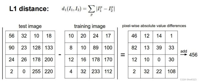
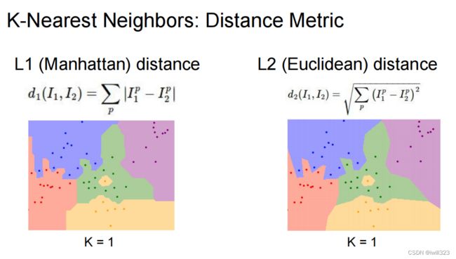
L1与L2距离
应用情况
数据集的划分
cross-validation
Linear Classifier
模型
实际意义
对权重矩阵的解释
对bias的处理
损失函数SVM loss
代码
Softmax classifier
Softmax vs. SVM
图像分类面临的问题
| Viewpoint variation | 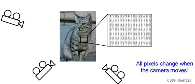 |
| Illumination |  |
| Background Clutter |  |
| Occlusion | 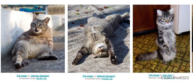 |
| Intraclass variation | 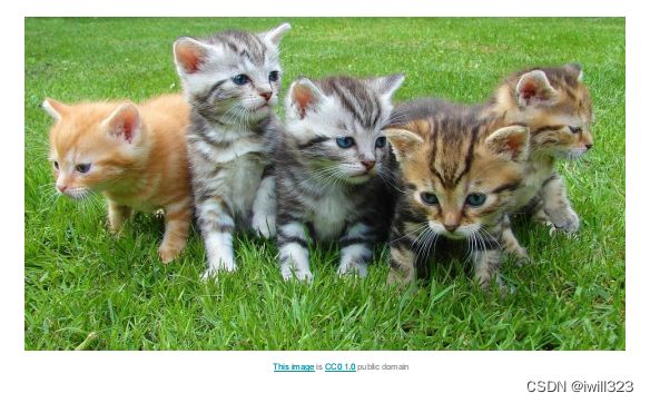 |
| Occlusion |  |
| Context | 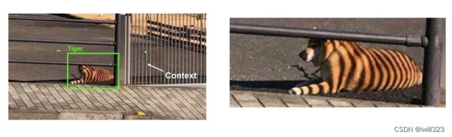 |
Machine Learning: Data-Driven Approach
我对Data-Driven的理解是:由算法自己从数据集中提取特征,用于分类
1. Collect a dataset of images and labels
2. Use Machine Learning algorithms to train a classifier
3. Evaluate the classifier on new images
K-Nearest Neighbor
原理
比较目标图片和每一个label集的图片每个位置对应的像素,相差值(求和)最小的那个label就是目标图片所属label
- During training, the classifier takes the training data and simply remembers it
- During testing, kNN classifies every test image by comparing to all training images and transfering the labels of the k most similar training examples
代码
以下代码出自官网CS231n Convolutional Neural Networks for Visual Recognition
import numpy as np

class NearestNeighbor(object):
  def __init__(self):
    pass

  def train(self, X, y):
    """
    X is N x D where each row is an example. Y is 1-dimension of size N
    """
    # the nearest neighbor classifier simply remembers all the training data
    self.Xtr = X
    self.ytr = y

  def predict(self, X):
    """
    X is N x D where each row is an example we wish to predict label for
    """
    num_test = X.shape[0]
    # lets make sure that the output type matches the input type
    Ypred = np.zeros(num_test, dtype = self.ytr.dtype)

    # loop over all test rows
    for i in range(num_test):
      # find the nearest training image to the i'th test image
      # using the L1 distance (sum of absolute value differences)
      distances = np.sum(np.abs(self.Xtr - X[i,:]), axis = 1)
      min_index = np.argmin(distances) # get the index with smallest distance
      Ypred[i] = self.ytr[min_index] # predict the label of the nearest example

    return Ypred
L2距离:
# 辅助函数
import numpy as np

class KNearestNeighbor(object):
    """ a kNN classifier with L2 distance """

    def __init__(self):
        pass

    def train(self, X, y):
        """
        Train the classifier. For k-nearest neighbors this is just memorizing the training data.

        Inputs:
        - X: A numpy array of shape (num_train, D) containing the training data
          consisting of num_train samples each of dimension D.
        - y: A numpy array of shape (N,) containing the training labels, where
             y[i] is the label for X[i].
        """
        self.X_train = X
        self.y_train = y

    def predict(self, X, k=1, num_loops=0):
        """
        Inputs:
        - X: A numpy array of shape (num_test, D) containing test data consisting
             of num_test samples each of dimension D.
        - k: The number of nearest neighbors that vote for the predicted labels.
        - num_loops: Determines which implementation to use to compute distances
          between training points and testing points.

        Returns:
        - y: A numpy array of shape (num_test,) containing predicted labels for the
          test data, where y[i] is the predicted label for the test point X[i].
        """
        dists = self.compute_distances(X)

        return self.predict_labels(dists, k=k)

    def compute_distances(self, X):
        num_test = X.shape[0]
        num_train = self.X_train.shape[0]
        dists = np.zeros((num_test, num_train))
        # (x - y)^2 = x^2 + y^2 - 2xy
        dists = np.sqrt(
            np.sum(X**2, axis=1,keepdims = True)
            - 2 * np.dot(X, self.X_train.T)
            + np.sum(X_train**2, axis = 1, keepdims = True).T
        )
return dists结果
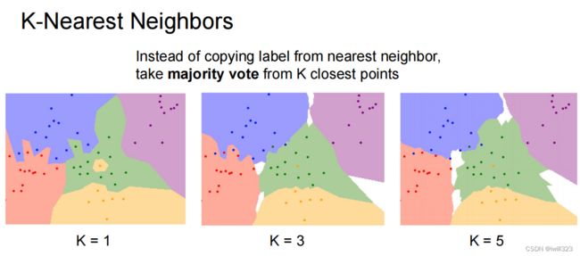
对于每个测试图片,找出得分最高的K个近邻点,然后看哪一个标签出现次数最多
- First we must compute the distances between all test examples and all train examples.
- Given these distances, for each test example we find the k nearest examples and have them vote for the label
# 辅助函数
import numpy as np

class KNearestNeighbor(object):
    """ a kNN classifier with L2 distance """

    def __init__(self):
        pass

    def train(self, X, y):
        """
        Train the classifier. For k-nearest neighbors this is just memorizing the training data.

        Inputs:
        - X: A numpy array of shape (num_train, D) containing the training data
          consisting of num_train samples each of dimension D.
        - y: A numpy array of shape (N,) containing the training labels, where
             y[i] is the label for X[i].
        """
        self.X_train = X
        self.y_train = y

    def predict(self, X, k=1, num_loops=0):
        """
        Inputs:
        - X: A numpy array of shape (num_test, D) containing test data consisting
             of num_test samples each of dimension D.
        - k: The number of nearest neighbors that vote for the predicted labels.
        - num_loops: Determines which implementation to use to compute distances
          between training points and testing points.

        Returns:
        - y: A numpy array of shape (num_test,) containing predicted labels for the
          test data, where y[i] is the predicted label for the test point X[i].
        """
        if num_loops == 0:
            dists = self.compute_distances_no_loops(X)
        elif num_loops == 1:
            dists = self.compute_distances_one_loop(X)
        elif num_loops == 2:
            dists = self.compute_distances_two_loops(X)
        else:
            raise ValueError("Invalid value %d for num_loops" % num_loops)

        return self.predict_labels(dists, k=k)

    def compute_distances_two_loops(self, X):
        """
        Inputs:
        - X: A numpy array of shape (num_test, D) containing test data.

        Returns:
        - dists: A numpy array of shape (num_test, num_train) where dists[i, j]
          is the Euclidean distance between the ith test point and the jth training
          point.
        """
        num_test = X.shape[0]
        num_train = self.X_train.shape[0]
        dists = np.zeros((num_test, num_train))
        for i in range(num_test):
            for j in range(num_train):
                dists[i,j] = np.sqrt(np.sum((X[i,:] - self.X_train[j, :]) **2))

        return dists

    def compute_distances_one_loop(self, X):
        """
        Compute the distance between each test point in X and each training point
        in self.X_train using a single loop over the test data.

        Input / Output: Same as compute_distances_two_loops
        """
        num_test = X.shape[0]
        num_train = self.X_train.shape[0]
        dists = np.zeros((num_test, num_train))
        for i in range(num_test):
            dists[i,:] = np.sqrt(((X[i,:] - self.X_train)**2).sum(1))
        return dists

    def compute_distances_no_loops(self, X):
        """
        Compute the distance between each test point in X and each training point
        in self.X_train using no explicit loops.

        Input / Output: Same as compute_distances_two_loops
        """
        num_test = X.shape[0]
        num_train = self.X_train.shape[0]
        dists = np.zeros((num_test, num_train))
        # (x - y)^2 = x^2 + y^2 - 2xy
        dists = np.sqrt(
            np.sum(X**2, axis=1,keepdims = True)
            + np.sum(self.X_train**2, axis = 1, keepdims = True).T
            - 2 * np.dot(X, self.X_train.T)
        )
        return dists
L1与L2距离
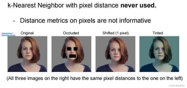
应用情况
主要原因是
- 预测花费的时间太长,不实用
- 图片背景的影响太大,容易遮住细节,而细节往往决定了图片最终的分类
数据集的划分
在训练集上尝试不同的超参数,在验证集上选择其中的最优超参数,在测试集上估算模型表现
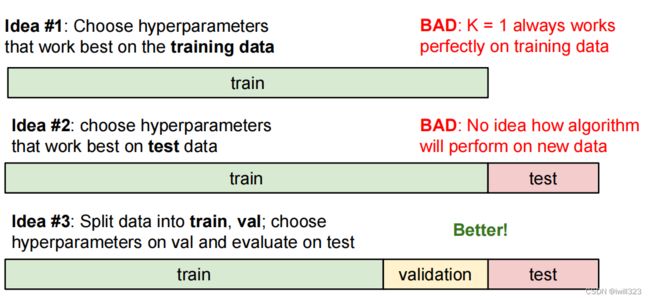
根据吴恩达的深度学习课程:
在小数据量的时代,如 100、1000、10000 的数据量大小,可以将数据集按照以下比例进行划分:
- 无验证集的情况:70% / 30%;
- 有验证集的情况:60% / 20% / 20%;
当数据非常多的时候
- 100 万数据量:98% / 1% / 1%;
- 超百万数据量:99.5% / 0.25% / 0.25%(或者99.5% / 0.4% / 0.1%)
cross-validation
当数据集比较小的时候,将其分成不同份数(比如5份),在其中四份上训练,在第五份上验证,调试超参数。然后选取其他fold作为验证集,如是共计操作5次
根据课程讲义:In practice, people prefer to avoid cross-validation in favor of having a single validation split, since cross-validation can be computationally expensive. If the number of examples in the validation set is small (perhaps only a few hundred or so), it is safer to use cross-validation
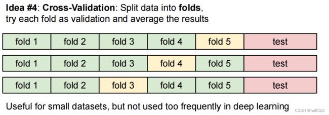
下面是5fold的示意图
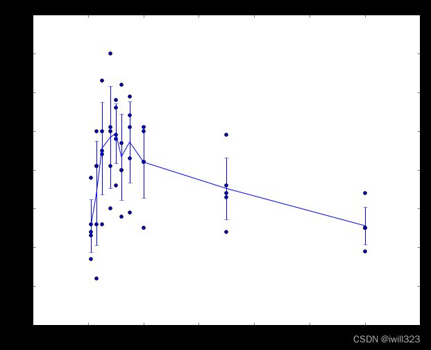
For each value of k we train on 4 folds and evaluate on the 5th. Hence, for each k we receive 5 accuracies on the validation fold (accuracy is the y-axis, each result is a point). The trend line is drawn through the average of the results for each k and the error bars indicate the standard deviation
num_folds = 5
k_choices = [1, 3, 5, 8, 10, 12, 15, 20, 50, 100]

X_train_folds = []
y_train_folds = []

# Split up the training data into folds. After splitting, X_train_folds and    #
# y_train_folds should each be lists of length num_folds, where                #
# y_train_folds[i] is the label vector for the points in X_train_folds[i].     #
X_train_folds = np.array_split(X_train, num_folds)
y_train_folds = np.array_split(y_train, num_folds)

# A dictionary holding the accuracies for different values of k that we find
# when running cross-validation.
k_to_accuracies = {}

# Perform k-fold cross validation to find the best value of k. For each        #
# possible value of k, run the k-nearest-neighbor algorithm num_folds times,   #
# where in each case you use all but one of the folds as training data and the #
# last fold as a validation set. Store the accuracies for all fold and all     #
# values of k in the k_to_accuracies dictionary.                               #
classifier = KNearestNeighbor()
for k in k_choices:
    k_to_accuracies[k] = []
    for i in range(num_folds):
        classifier.train(np.concatenate(np.delete(X_train_folds, i, 0)),
                         np.concatenate(np.delete(y_train_folds, i, 0)))
        y_test_pred = classifier.predict(X_train_folds[i], k=k)
        k_to_accuracies[k].append(np.mean(y_test_pred == y_train_folds[i]))

# Print out the computed accuracies
for k in sorted(k_to_accuracies):
    for accuracy in k_to_accuracies[k]:
        print('k = %d, accuracy = %f' % (k, accuracy))
代码:K近邻法和Cross-validation_iwill323的博客-CSDN博客
Linear Classifier
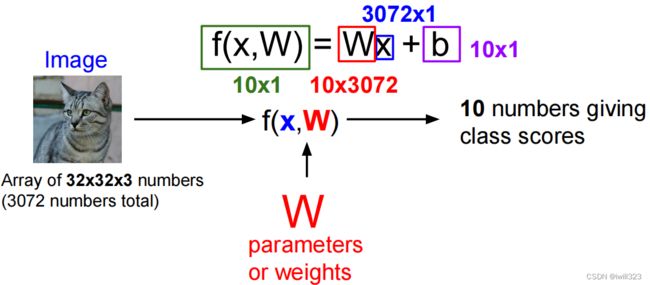
模型
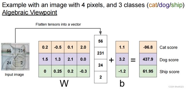
将输入图像伸展为列向量x,大小为[D×1],权重矩阵W大小[K×D],这样Wx的结果就是[K×1]的矩阵,对应着该图像在K类上的得分score
w的形状:标签数 * 特征数
x的形状: 特征数 * 样本量
实际意义
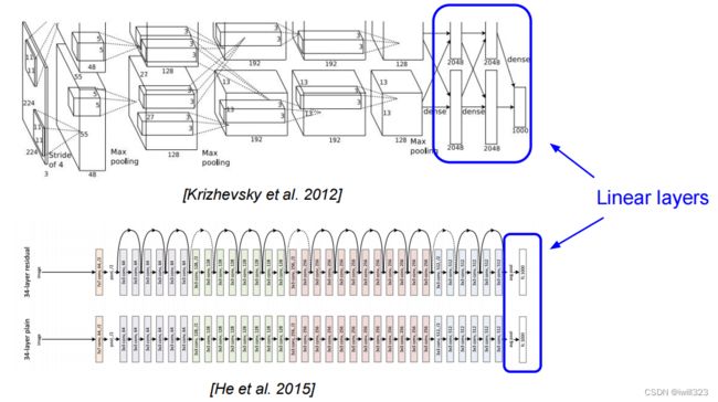
在卷积神经网络的末端,经常使用全连接层将提取到的图像特征转化为分类得分
对权重矩阵的解释
下图是CIFAR-10学习到的权重矩阵。W每一行对应着每一类的样本template(也叫prototype)。一个图片在每个分类上的得分就是将图像和每个template做内积的结果。线性分类器的所做的就是template matching。换种角度,其实这里做的和K-Nearest类似,差别在于图片不是和数据集里成百上千的图片比对,而是和一个个template比对。并且,使用的是内积而不是L1或L2距离
我觉得可以从激活的角度考虑:当图像的点和template在分布上接近的时候,乘积结果更大
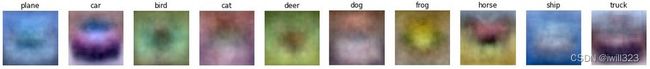
Note that, for example, the ship template contains a lot of blue pixels as expected. This template will therefore give a high score once it is matched against images of ships on the ocean with an inner product.
对bias的处理
一种简化计算的方法是将bias作为权重的一个维度加入权重

损失函数SVM loss
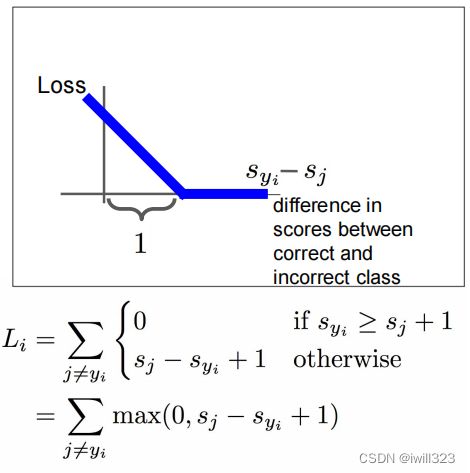
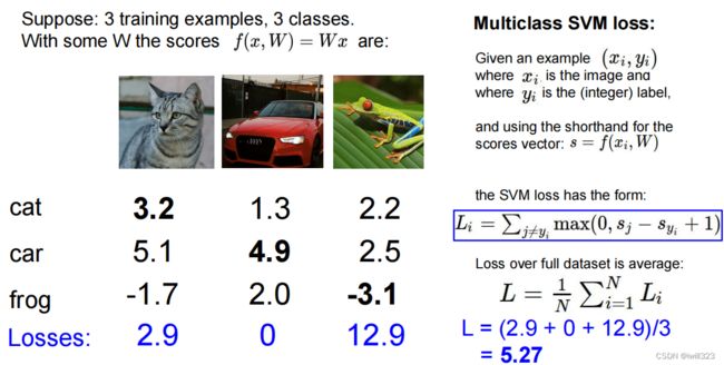
Q1:what is the min/max possible SVM loss Li?
Ans: 0/ inf
Ans: C
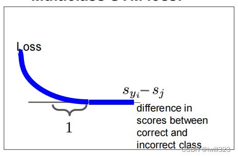
Ans:对大偏移量的惩罚更大
代码
来自官网CS231n Convolutional Neural Networks for Visual Recognition
def L_i_vectorized(x, y, W):
  """
  A faster half-vectorized implementation. half-vectorized
  refers to the fact that for a single example the implementation contains
  no for loops, but there is still one loop over the examples (outside this function)
  """
  delta = 1.0
  scores = W.dot(x)
  # compute the margins for all classes in one vector operation
  margins = np.maximum(0, scores - scores[y] + delta)
  # on y-th position scores[y] - scores[y] canceled and gave delta. We want
  # to ignore the y-th position and only consider margin on max wrong class
  margins[y] = 0
  loss_i = np.sum(margins)
  return loss_i
def svm_loss_vectorized(W, X, y, reg):
"""
Structured SVM loss function, vectorized implementation.
"""
loss = 0.0
dW = np.zeros(W.shape) # initialize the gradient as zero
scores = X.dot(W) # N, C
num_class = W.shape[1]
num_train = X.shape[0]
correct_class_score = scores[np.arange(num_train), y] # shape: (num_class,)
correct_class_score = correct_class_score.reshape([-1, 1]) # shape: (num_class,1)
loss_tep = scores - correct_class_score + 1
loss_tep[loss_tep < 0] = 0 # 求与0相比的最大值
# loss_tep = np.maximum(0, loss_tep)
loss_tep[np.arange(num_train), y] = 0 # 正确的类loss为0
loss = loss_tep.sum()/num_train + reg * np.sum(W * W)
# loss_tep元素大于0的位置说明此处有loss,对于非正确标签类求导为1
loss_tep[loss_tep > 0] = 1 # N, C
# 对于正确标签类,每有一个loss_tep元素大于0,则正确标签类求导为-1,要累加
loss_item_count = np.sum(loss_tep, axis=1)
loss_tep[np.arange(num_train), y] -= loss_item_count #在一次错误的分类中,
# dW中第i,j元素对应于第i维,第j类的权重
# X.T的第i行每个元素对应于每个样本第i维的输入,正是Sj对W[i,j]的导数
# loss_tep的第j列每个元素对应于每个样本在第j类的得分是否出现,相当于掩码
# X.T和loss_tep的矩阵乘法等于对每个样本的W[i,j]导数值求和
dW = X.T.dot(loss_tep) / num_train # (D, N) *(N, C)
dW += 2 * reg * W
return loss, dW# inear_classifier.py.
class LinearClassifier(object):
def __init__(self):
self.W = None
def train(
self,
X,
y,
learning_rate=1e-3,
reg=1e-5,
num_iters=100,
batch_size=200,
verbose=False,
):
"""
Train this linear classifier using stochastic gradient descent.
Inputs:
- X: A numpy array of shape (N, D) containing training data; there are N
training samples each of dimension D.
- y: A numpy array of shape (N,) containing training labels; y[i] = c
means that X[i] has label 0 <= c < C for C classes.
- learning_rate: (float) learning rate for optimization.
- reg: (float) regularization strength.
- num_iters: (integer) number of steps to take when optimizing
- batch_size: (integer) number of training examples to use at each step.
- verbose: (boolean) If true, print progress during optimization.
Outputs:
A list containing the value of the loss function at each training iteration.
"""
num_train, dim = X.shape
num_classes = (
np.max(y) + 1
) # assume y takes values 0...K-1 where K is number of classes
if self.W is None:
# lazily initialize W
self.W = 0.001 * np.random.randn(dim, num_classes)
# Run stochastic gradient descent to optimize W
loss_history = []
for it in range(num_iters):
X_batch = None
y_batch = None
mask = np.random.choice(num_train, batch_size, replace=True)
# replace=True代表选出来的样本可以重复。
# 每次迭代都是重新随机选样本组成batch,意味着有些会选不到,有点会被重复选。有些粗糙
X_batch = X[mask]
y_batch = y[mask]
# evaluate loss and gradient
loss, grad = self.loss(X_batch, y_batch, reg)
loss_history.append(loss)
self.W -= learning_rate * grad
if verbose and it % 100 == 0:
print("iteration %d / %d: loss %f" % (it, num_iters, loss))
return loss_history
def predict(self, X):
"""
Use the trained weights of this linear classifier to predict labels for
data points.
Inputs:
- X: A numpy array of shape (N, D) containing training data; there are N
training samples each of dimension D.
Returns:
- y_pred: Predicted labels for the data in X. y_pred is a 1-dimensional
array of length N, and each element is an integer giving the predicted
class.
"""
y_pred = np.zeros(X.shape[0])
y_pred = np.argmax(X.dot(self.W), axis = 1) # (N, D) * (D, C)
return y_pred
def loss(self, X_batch, y_batch, reg):
"""
Compute the loss function and its derivative.
Subclasses will override this.
"""
pass
class LinearSVM(LinearClassifier):
""" A subclass that uses the Multiclass SVM loss function """
def loss(self, X_batch, y_batch, reg):
return svm_loss_vectorized(self.W, X_batch, y_batch, reg)
svm = LinearSVM()
tic = time.time()
loss_hist = svm.train(X_train, y_train, learning_rate=1e-7, reg=2.5e4,
num_iters=1500, verbose=True)
toc = time.time()
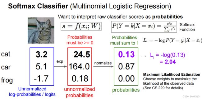
print('That took %fs' % (toc - tic))Softmax classifier
特点是,将原始的分类得分转化为对应的可能性 interpret raw classifier scores as probabilities,且所有可能性的总和是1
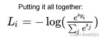
 公式:
公式:
def softmax_loss_vectorized(W, X, y, reg):
    """
    Softmax loss function, vectorized version.

    Inputs and outputs are the same as softmax_loss_naive.
    """
    # Initialize the loss and gradient to zero.
    loss = 0.0
    dW = np.zeros_like(W)

    num_trains = X.shape[0]
    num_calss = W.shape[1]
    scores = X.dot(W)  # (N, C)
    max_val = np.max(scores, axis=1).reshape(-1, 1) # 求每一个样本中的最大得分
    f = scores - max_val # 防止指数过大,计算溢出
    softmax = np.exp(f)/ np.exp(f).sum(axis=1).reshape(-1,1)
    loss_i = -np.log(softmax[np.arange(num_trains), y]).sum() # 将分类正确的softmax取出
    loss += loss_i

    softmax[np.arange(num_trains), y] -= 1  #处理log的分子项的导数
    dW = X.T.dot(softmax)  # dW[:, j] += X[i] * softmax[j]的向量化

    loss /= num_trains
    dW /= num_trains

    loss += reg * np.sum(W * W)
    dW += 2 * reg * W
    # *****END OF YOUR CODE (DO NOT DELETE/MODIFY THIS LINE)*****

    return loss, dW
Softmax vs. SVM
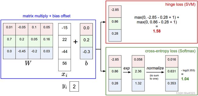
The difference is in the interpretation of the scores in f:
The SVM interprets these as class scores and its loss function encourages the correct class (class 2, in blue) to have a score higher by a margin than the other class scores. 只要正确标签的得分比错误标签足够大就满足了,在此基础上,正确标签得分高一点低一点对loss都没有影响
The Softmax classifier instead interprets the scores as (unnormalized) log probabilities for each class and then encourages the (normalized) log probability of the correct class to be high (equivalently the negative of it to be low). Softmax 分类器的目标是让正确标签得分越高越好
代码:线性分类器(SVM,softmax)_iwill323的博客-CSDN博客
K近邻法和Cross-validation_iwill323的博客-CSDN博客