Neural Networks and Deep Learning week2 Python Basics with numpy (optional)

该实验作业的主要目的

1. 熟悉使用jupyterlab来编写python代码
2. sigmoid
3. numpy一些函数的使用
4. shape和reshape修改向量
5. python的广播特性
6. 向量化代码以减少循环loop
7. numpy的帮助文件 https://numpy.org/doc/stable/index.html

总体进程

热身 写一个hello world

1.1 写一个sigmoid函数

当我们将该sigmoid函数进行移植时发现太局限，无法对数组等进行运算，因而我们需要对此进行修改

1.1 用numpy重构一个sigmoid函数

从最直观的梯度开始对函数参数进行修改

1.2 完成对sigmoid函数的求导

我们将要对图片进行分类，然而图像分为RGB三层，现在我们需要对图片进行大小转化

1.3使用shape将矩阵转换为列向量

1.4 标准化向量（数据规范化，回想以前的梯度过程，规范化可以让迭代更迅速，迭代图像更加圆润而非一条近似直线）

1.5 使用python的广播特性

2向量化

今后我们要面对很多很大的数据，如果仍按照以前的循环方式，这对工程很麻烦，好在我们由很多矩阵快速算法，因而我们需要想办法将数据向量化

2.1 完成损失函数

在需要写代码的前面我将提示任务目标

Python Basics with Numpy (optional assignment)

Welcome to your first assignment. This exercise gives you a brief introduction to Python. Even if you've used Python before, this will help familiarize you with functions we'll need.

Instructions:

• You will be using Python 3.
• Avoid using for-loops and while-loops, unless you are explicitly told to do so.
• Do not modify the (# GRADED FUNCTION [function name]) comment in some cells. Your work would not be graded if you change this. Each cell containing that comment should only contain one function.
• After coding your function, run the cell right below it to check if your result is correct.

After this assignment you will:

• Be able to use iPython Notebooks
• Be able to use numpy functions and numpy matrix/vector operations
• Understand the concept of "broadcasting"
• Be able to vectorize code

Let's get started!

Updates to Assignment

This is version 3a of the notebook.

If you were working on a previous version

• If you were already working on version "3", you'll find your original work in the file directory.
• To reach the file directory, click on the "Coursera" icon in the top left of this notebook.
• Please still use the most recent notebook to submit your assignment.

List of Updates

• softmax section has a comment to clarify the use of "m" later in the course
• softmax function specifies (m,n) matrix dimensions to match the notation in the preceding diagram (instead of n,m)

About iPython Notebooks

iPython Notebooks are interactive coding environments embedded in a webpage. You will be using iPython notebooks in this class. You only need to write code between the ### START CODE HERE ### and ### END CODE HERE ### comments. After writing your code, you can run the cell by either pressing "SHIFT"+"ENTER" or by clicking on "Run Cell" (denoted by a play symbol) in the upper bar of the notebook.

We will often specify "(≈ X lines of code)" in the comments to tell you about how much code you need to write. It is just a rough estimate, so don't feel bad if your code is longer or shorter.

Exercise: Set test to "Hello World" in the cell below to print "Hello World" and run the two cells below.

现实一个字符串  Hello World

### START CODE HERE ### (≈ 1 line of code)
test = "Hello World"
### END CODE HERE ###
print ("test: " + test)

Expected output: test: Hello World

**What you need to remember**: - Run your cells using SHIFT+ENTER (or "Run cell") - Write code in the designated areas using Python 3 only - Do not modify the code outside of the designated areas

1 - Building basic functions with numpy

Numpy is the main package for scientific computing in Python. It is maintained by a large community (www.numpy.org). In this exercise you will learn several key numpy functions such as np.exp, np.log, and np.reshape. You will need to know how to use these functions for future assignments.

1.1 - sigmoid function, np.exp()

Before using np.exp(), you will use math.exp() to implement the sigmoid function. You will then see why np.exp() is preferable to math.exp().

Exercise: Build a function that returns the sigmoid of a real number x. Use math.exp(x) for the exponential function.

Reminder: ()= is sometimes also known as the logistic function. It is a non-linear function used not only in Machine Learning (Logistic Regression), but also in Deep Learning.

To refer to a function belonging to a specific package you could call it using package_name.function(). Run the code below to see an example with math.exp().

完成sigmoid函数  使用 math.exp(x)以完成指数运算

# GRADED FUNCTION: basic_sigmoid

import math

def basic_sigmoid(x):
    """
    Compute sigmoid of x.

    Arguments:
    x -- A scalar

    Return:
    s -- sigmoid(x)
    """
    
    ### START CODE HERE ### (≈ 1 line of code)
    s = None
    s = 1 / (1 + math.exp(-x) )
    ### END CODE HERE ###
    
    return s

basic_sigmoid(3)

Expected Output:

basic_sigmoid(3)

0.9525741268224334

Actually, we rarely use the "math" library in deep learning because the inputs of the functions are real numbers. In deep learning we mostly use matrices and vectors. This is why numpy is more useful.

### One reason why we use "numpy" instead of "math" in Deep Learning ###
x = [1, 2, 3]
basic_sigmoid(x) # you will see this give an error when you run it, because x is a vector.

---------------------------------------------------------------------------
TypeError                                 Traceback (most recent call last)
 in ()
      1 ### One reason why we use "numpy" instead of "math" in Deep Learning ###
      2 x = [1, 2, 3]
----> 3 basic_sigmoid(x) # you will see this give an error when you run it, because x is a vector.

 in basic_sigmoid(x)
     16     ### START CODE HERE ### (≈ 1 line of code)
     17     s = None
---> 18     s = 1 / (1 + math.exp(-x) )
     19     ### END CODE HERE ###
     20 

TypeError: bad operand type for unary -: 'list'

In fact, if  is a row vector then np.exp(x) will apply the exponential function to every element of x. The output will thus be: np.exp(x)=

import numpy as np

# example of np.exp
x = np.array([1, 2, 3])
print(np.exp(x)) # result is (exp(1), exp(2), exp(3))

Furthermore, if x is a vector, then a Python operation such as s=x+3 or will output s as a vector of the same size as x.

# example of vector operation
x = np.array([1, 2, 3])
print (x + 3)

Any time you need more info on a numpy function, we encourage you to look at the official documentation.

You can also create a new cell in the notebook and write np.exp? (for example) to get quick access to the documentation.

Exercise: Implement the sigmoid function using numpy.

Instructions: x could now be either a real number, a vector, or a matrix. The data structures we use in numpy to represent these shapes (vectors, matrices...) are called numpy arrays. You don't need to know more for now.

 

For x∈ℝn, 

由于上面的那个简单sigmoid应用不广泛，仅能用于单变量，无法用于矩阵，现在我们开始尝试numpy的函数

# GRADED FUNCTION: sigmoid

import numpy as np # this means you can access numpy functions by writing np.function() instead of numpy.function()

def sigmoid(x):
    """
    Compute the sigmoid of x

    Arguments:
    x -- A scalar or numpy array of any size

    Return:
    s -- sigmoid(x)
    """
    
    ### START CODE HERE ### (≈ 1 line of code)
    s = None
    s = 1/(1+np.exp(-x))
    ### END CODE HERE ###
    
    return s

x = np.array([1, 2, 3])
sigmoid(x)

Expected Output:

sigmoid([1,2,3])

array([ 0.73105858, 0.88079708, 0.95257413])

1.2 - Sigmoid gradient

As you've seen in lecture, you will need to compute gradients to optimize loss functions using backpropagation. Let's code your first gradient function.

Exercise: Implement the function sigmoid_grad() to compute the gradient of the sigmoid function with respect to its input x. The formula is:

sigmoid_derivative(x)=σ′(x)=σ(x)(1−σ(x))     (2)

You often code this function in two steps:

1. Set s to be the sigmoid of x. You might find your sigmoid(x) function useful.
2. Compute σ′(x)=s(1−s)

# GRADED FUNCTION: sigmoid_derivative

def sigmoid_derivative(x):
    """
    Compute the gradient (also called the slope or derivative) of the sigmoid function with respect to its input x.
    You can store the output of the sigmoid function into variables and then use it to calculate the gradient.
    
    Arguments:
    x -- A scalar or numpy array

    Return:
    ds -- Your computed gradient.
    """
    
    ### START CODE HERE ### (≈ 2 lines of code)
    s = sigmoid(x)
    ds = s * ( 1 - s )
    ### END CODE HERE ###
    
    return ds

x = np.array([1, 2, 3])
print ("sigmoid_derivative(x) = " + str(sigmoid_derivative(x)))

Expected Output:

sigmoid_derivative([1,2,3])

[ 0.19661193 0.10499359 0.04517666]

1.3 - Reshaping arrays

Two common numpy functions used in deep learning are np.shape and np.reshape().

• X.shape is used to get the shape (dimension) of a matrix/vector X.
• X.reshape(...) is used to reshape X into some other dimension.

For example, in computer science, an image is represented by a 3D array of shape (length,height,depth=3)(length,height,depth=3). However, when you read an image as the input of an algorithm you convert it to a vector of shape (length∗height∗3,1)(length∗height∗3,1). In other words, you "unroll", or reshape, the 3D array into a 1D vector.

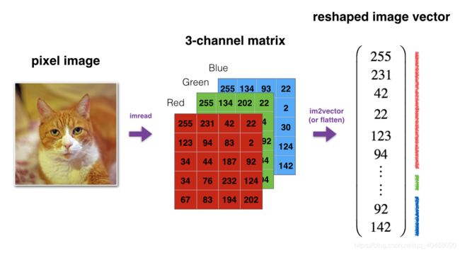
Exercise: Implement image2vector() that takes an input of shape (length, height, 3) and returns a vector of shape (length*height*3, 1). For example, if you would like to reshape an array v of shape (a, b, c) into a vector of shape (a*b,c) you would do:

v = v.reshape((v.shape[0]*v.shape[1], v.shape[2])) # v.shape[0] = a ; v.shape[1] = b ; v.shape[2] = c

• Please don't hardcode the dimensions of image as a constant. Instead look up the quantities you need with image.shape[0], etc.

# GRADED FUNCTION: image2vector
def image2vector(image):
    """
    Argument:
    image -- a numpy array of shape (length, height, depth)
    
    Returns:
    v -- a vector of shape (length*height*depth, 1)
    """
    
    ### START CODE HERE ### (≈ 1 line of code)
    v = image.reshape(image.shape[0]*image.shape[1]*image.shape[2],1)
    ### END CODE HERE ###
    
    return v

# This is a 3 by 3 by 2 array, typically images will be (num_px_x, num_px_y,3) where 3 represents the RGB values
image = np.array([[[ 0.67826139,  0.29380381],
        [ 0.90714982,  0.52835647],
        [ 0.4215251 ,  0.45017551]],

       [[ 0.92814219,  0.96677647],
        [ 0.85304703,  0.52351845],
        [ 0.19981397,  0.27417313]],

       [[ 0.60659855,  0.00533165],
        [ 0.10820313,  0.49978937],
        [ 0.34144279,  0.94630077]]])

print ("image2vector(image) = " + str(image2vector(image)))

Expected Output:

image2vector(image)

[[ 0.67826139] [ 0.29380381] [ 0.90714982] [ 0.52835647] [ 0.4215251 ] [ 0.45017551] [ 0.92814219] [ 0.96677647] [ 0.85304703] [ 0.52351845] [ 0.19981397] [ 0.27417313] [ 0.60659855] [ 0.00533165] [ 0.10820313] [ 0.49978937] [ 0.34144279] [ 0.94630077]]

1.4 - Normalizing rows

Another common technique we use in Machine Learning and Deep Learning is to normalize our data. It often leads to a better performance because gradient descent converges faster after normalization. Here, by normalization we mean changing x to  (dividing each row vector of x by its norm).

For example, if

then

∥x∥=np.linalg.norm(x,axis=1,keepdims=True)=(4)

and

=

Note that you can divide matrices of different sizes and it works fine: this is called broadcasting and you're going to learn about it in part 5.

Exercise: Implement normalizeRows() to normalize the rows of a matrix. After applying this function to an input matrix x, each row of x should be a vector of unit length (meaning length 1).

实现标准化矩阵

# GRADED FUNCTION: normalizeRows

def normalizeRows(x):
    """
    Implement a function that normalizes each row of the matrix x (to have unit length).
    
    Argument:
    x -- A numpy matrix of shape (n, m)
    
    Returns:
    x -- The normalized (by row) numpy matrix. You are allowed to modify x.
    """
    
    ### START CODE HERE ### (≈ 2 lines of code)
    # Compute x_norm as the norm 2 of x. Use np.linalg.norm(..., ord = 2, axis = ..., keepdims = True)
    x_norm = np.linalg.norm(x,axis=1,keepdims=True)
    
    # Divide x by its norm.
    x = x/x_norm
    ### END CODE HERE ###

    return x

x = np.array([
    [0, 3, 4],
    [1, 6, 4]])
print("normalizeRows(x) = " + str(normalizeRows(x)))

Expected Output:

normalizeRows(x)

[[ 0. 0.6 0.8 ] [ 0.13736056 0.82416338 0.54944226]]

Note: In normalizeRows(), you can try to print the shapes of x_norm and x, and then rerun the assessment. You'll find out that they have different shapes. This is normal given that x_norm takes the norm of each row of x. So x_norm has the same number of rows but only 1 column. So how did it work when you divided x by x_norm? This is called broadcasting and we'll talk about it now!

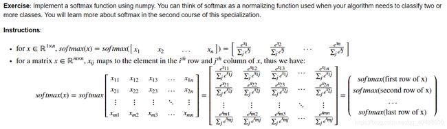
1.5 - Broadcasting and the softmax function

A very important concept to understand in numpy is "broadcasting". It is very useful for performing mathematical operations between arrays of different shapes. For the full details on broadcasting, you can read the official broadcasting documentation.

Note

Note that later in the course, you'll see "m" used to represent the "number of training examples", and each training example is in its own column of the matrix.
Also, each feature will be in its own row (each row has data for the same feature).
Softmax should be performed for all features of each training example, so softmax would be performed on the columns (once we switch to that representation later in this course).

However, in this coding practice, we're just focusing on getting familiar with Python, so we're using the common math notation m×nm×n
where mm is the number of rows and n is the number of columns.

实现矩阵的标准化

# GRADED FUNCTION: softmax

def softmax(x):
    """Calculates the softmax for each row of the input x.

    Your code should work for a row vector and also for matrices of shape (m,n).

    Argument:
    x -- A numpy matrix of shape (m,n)

    Returns:
    s -- A numpy matrix equal to the softmax of x, of shape (m,n)
    """
    
    ### START CODE HERE ### (≈ 3 lines of code)
    # Apply exp() element-wise to x. Use np.exp(...).
    x_exp = np.exp(x)

    # Create a vector x_sum that sums each row of x_exp. Use np.sum(..., axis = 1, keepdims = True).
    x_sum = np.sum(x_exp,axis=1,keepdims=True)
    
    # Compute softmax(x) by dividing x_exp by x_sum. It should automatically use numpy broadcasting.
    s = x_exp/x_sum

    ### END CODE HERE ###
    
    return s

x = np.array([
    [9, 2, 5, 0, 0],
    [7, 5, 0, 0 ,0]])
print("softmax(x) = " + str(softmax(x)))

Expected Output:

softmax(x)

[[ 9.80897665e-01 8.94462891e-04 1.79657674e-02 1.21052389e-04 1.21052389e-04] [ 8.78679856e-01 1.18916387e-01 8.01252314e-04 8.01252314e-04 8.01252314e-04]]

Note:

• If you print the shapes of x_exp, x_sum and s above and rerun the assessment cell, you will see that x_sum is of shape (2,1) while x_exp and s are of shape (2,5). x_exp/x_sum works due to python broadcasting.

Congratulations! You now have a pretty good understanding of python numpy and have implemented a few useful functions that you will be using in deep learning.

What you need to remember:

• np.exp(x) works for any np.array x and applies the exponential function to every coordinate
• the sigmoid function and its gradient
• image2vector is commonly used in deep learning
• np.reshape is widely used. In the future, you'll see that keeping your matrix/vector dimensions straight will go toward eliminating a lot of bugs.
• numpy has efficient built-in functions
• broadcasting is extremely useful

2) Vectorization

In deep learning, you deal with very large datasets. Hence, a non-computationally-optimal function can become a huge bottleneck in your algorithm and can result in a model that takes ages to run. To make sure that your code is computationally efficient, you will use vectorization. For example, try to tell the difference between the following implementations of the dot/outer/elementwise product.

import time

x1 = [9, 2, 5, 0, 0, 7, 5, 0, 0, 0, 9, 2, 5, 0, 0]
x2 = [9, 2, 2, 9, 0, 9, 2, 5, 0, 0, 9, 2, 5, 0, 0]

### CLASSIC DOT PRODUCT OF VECTORS IMPLEMENTATION ###
tic = time.process_time()
dot = 0
for i in range(len(x1)):
    dot+= x1[i]*x2[i]
toc = time.process_time()
print ("dot = " + str(dot) + "\n ----- Computation time = " + str(1000*(toc - tic)) + "ms")

### CLASSIC OUTER PRODUCT IMPLEMENTATION ###
tic = time.process_time()
outer = np.zeros((len(x1),len(x2))) # we create a len(x1)*len(x2) matrix with only zeros
for i in range(len(x1)):
    for j in range(len(x2)):
        outer[i,j] = x1[i]*x2[j]
toc = time.process_time()
print ("outer = " + str(outer) + "\n ----- Computation time = " + str(1000*(toc - tic)) + "ms")

### CLASSIC ELEMENTWISE IMPLEMENTATION ###
tic = time.process_time()
mul = np.zeros(len(x1))
for i in range(len(x1)):
    mul[i] = x1[i]*x2[i]
toc = time.process_time()
print ("elementwise multiplication = " + str(mul) + "\n ----- Computation time = " + str(1000*(toc - tic)) + "ms")

### CLASSIC GENERAL DOT PRODUCT IMPLEMENTATION ###
W = np.random.rand(3,len(x1)) # Random 3*len(x1) numpy array
tic = time.process_time()
gdot = np.zeros(W.shape[0])
for i in range(W.shape[0]):
    for j in range(len(x1)):
        gdot[i] += W[i,j]*x1[j]
toc = time.process_time()
print ("gdot = " + str(gdot) + "\n ----- Computation time = " + str(1000*(toc - tic)) + "ms")

dot = 278
 ----- Computation time = 0.08973300000003626ms

---------------------------------------------------------------------------
NameError                                 Traceback (most recent call last)
 in ()
     14 ### CLASSIC OUTER PRODUCT IMPLEMENTATION ###
     15 tic = time.process_time()
---> 16 outer = np.zeros((len(x1),len(x2))) # we create a len(x1)*len(x2) matrix with only zeros
     17 for i in range(len(x1)):
     18     for j in range(len(x2)):

NameError: name 'np' is not defined

x1 = [9, 2, 5, 0, 0, 7, 5, 0, 0, 0, 9, 2, 5, 0, 0]
x2 = [9, 2, 2, 9, 0, 9, 2, 5, 0, 0, 9, 2, 5, 0, 0]

### VECTORIZED DOT PRODUCT OF VECTORS ###
tic = time.process_time()
dot = np.dot(x1,x2)
toc = time.process_time()
print ("dot = " + str(dot) + "\n ----- Computation time = " + str(1000*(toc - tic)) + "ms")

### VECTORIZED OUTER PRODUCT ###
tic = time.process_time()
outer = np.outer(x1,x2)
toc = time.process_time()
print ("outer = " + str(outer) + "\n ----- Computation time = " + str(1000*(toc - tic)) + "ms")

### VECTORIZED ELEMENTWISE MULTIPLICATION ###
tic = time.process_time()
mul = np.multiply(x1,x2)
toc = time.process_time()
print ("elementwise multiplication = " + str(mul) + "\n ----- Computation time = " + str(1000*(toc - tic)) + "ms")

### VECTORIZED GENERAL DOT PRODUCT ###
tic = time.process_time()
dot = np.dot(W,x1)
toc = time.process_time()
print ("gdot = " + str(dot) + "\n ----- Computation time = " + str(1000*(toc - tic)) + "ms")

As you may have noticed, the vectorized implementation is much cleaner and more efficient. For bigger vectors/matrices, the differences in running time become even bigger.

Note that np.dot() performs a matrix-matrix or matrix-vector multiplication. This is different from np.multiply() and the * operator (which is equivalent to .* in Matlab/Octave), which performs an element-wise multiplication.

2.1 Implement the L1 and L2 loss functions

Exercise: Implement the numpy vectorized version of the L1 loss. You may find the function abs(x) (absolute value of x) useful.

Reminder:

• The loss is used to evaluate the performance of your model. The bigger your loss is, the more different your predictions (ŷ y^) are from the true values (yy). In deep learning, you use optimization algorithms like Gradient Descent to train your model and to minimize the cost.
• L1 loss is defined as:

  
  

计算偏差

# GRADED FUNCTION: L1

def L1(yhat, y):
    """
    Arguments:
    yhat -- vector of size m (predicted labels)
    y -- vector of size m (true labels)
    
    Returns:
    loss -- the value of the L1 loss function defined above
    """
    
    ### START CODE HERE ### (≈ 1 line of code)
    loss = np.sum(np.abs(y-yhat))
    ### END CODE HERE ###
    
    return loss

yhat = np.array([.9, 0.2, 0.1, .4, .9])
y = np.array([1, 0, 0, 1, 1])
print("L1 = " + str(L1(yhat,y)))

Expected Output:

L1

1.1

Exercise: Implement the numpy vectorized version of the L2 loss. There are several way of implementing the L2 loss but you may find the function np.dot() useful. As a reminder, if x=[x1,x2,...,xn]x=[x1,x2,...,xn], then np.dot(x,x) = 

• L2 loss is defined as

  

计算代价函数J

# GRADED FUNCTION: L2

def L2(yhat, y):
    """
    Arguments:
    yhat -- vector of size m (predicted labels)
    y -- vector of size m (true labels)
    
    Returns:
    loss -- the value of the L2 loss function defined above
    """
    
    ### START CODE HERE ### (≈ 1 line of code)
    loss = np.sum(pow(y-yhat,2))
    ### END CODE HERE ###
    
    return loss

yhat = np.array([.9, 0.2, 0.1, .4, .9])
y = np.array([1, 0, 0, 1, 1])
print("L2 = " + str(L2(yhat,y)))

Expected Output:

L2

0.43

 

Congratulations on completing this assignment. We hope that this little warm-up exercise helps you in the future assignments, which will be more exciting and interesting!

 

What to remember:

• Vectorization is very important in deep learning. It provides computational efficiency and clarity.
• You have reviewed the L1 and L2 loss.
• You are familiar with many numpy functions such as np.sum, np.dot, np.multiply, np.maximum, etc...