图解注意力机制
- 数十年以来,统计机器翻译(Statistical Machine Translation)在翻译模型中占统治地位,直到出现神经机器翻译(Neural Machine Translate,NMT)。NMT是一种新兴机器翻译方法,意图构建和训练一种大型神经网络,输入原语言文本(source),输出目标翻译文本(target)。
- NMT最初是由Kalchbrenner and Blunsom(2013), Sutskever et. al (2014) and Cho. et. al (2014b)提出,其中大家最熟悉的框架就是Sutskever的sequence-to-sequence(seq2seq)网络结构。这篇博客也是基于seq2seq经典框架进行剖析以及怎么实现注意力机制的。
PART 1:综述
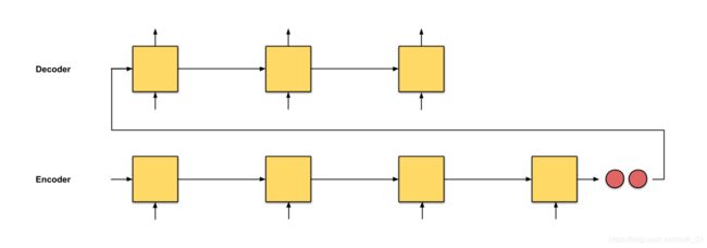
Fig. 0.1: seq2seq with an input sequence of length 4
在seq2seq中,其思想就是构造两个循环神经网络(RNNs),就是编码器和解码器。
-
encoder:处理输入序列,把信息压缩成一个有固定维度的context vector(也成为sentence embedding或者“thought” vector)。这个向量代表了整个源句子输入的语义表示。
-
decoder:由编码器输出的context vector初始化,‘********,在早期的工作中,使用了编码器网络的最后一个隐状态作为解码器的初始隐状态。

Fig. 3. The encoder-decoder model, translating the sentence “she is eating a green apple” to Chinese. The visualization of both encoder and decoder is unrolled in time.
很清楚,这种定长的context vector设计有个很致命的问题,无法记忆长句子。当处理完所有输入序列后,模型对最初的输入单词已经**“忘得差不多了”**。也就是编码器输出的context vector并不能很好地表征长句子的开头部分信息。所以注意力机制就是为了解决这个问题提出的。
最初提出注意力机制就是为了解决神经机器翻译任务中长的源句子的记忆问题。注意力机制的做法并不要创建一个与编码器最后一个隐状态(last hidden state)完全无关的context vector,而是要创建一个与编码器所有的隐状态有关的 加权 context vector,当然也包括 最后一个隐状态(这就是所谓global attention)。
现在context vector 能遍历整个输入序列,所以我们不用担心遗忘的问题。接下来就要学习源语言和目标语言之间的对齐,这种对齐由context vector控制。
对齐(alignment)
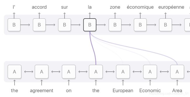
对齐就是把原始文本的单词(也可能是一段)和翻译所对应的单词相匹配,如图所示。
Fig. 0.3: Alignment for the French word ‘la’ is distributed across the input sequence but mainly on these 4 words: ‘the’, ‘European’, ‘Economic’ and ‘Area’. Darker purple indicates better attention scores (Image source)
下面重点讲解加入注意力机制的context vector到底由什么组成,主要分下面三个部分:
- 编码器的隐状态
- 解码器的隐状态
- source和target之间的对齐

Fig. 4. The encoder-decoder model with additive attention mechanism in Bahdanau et al., 2015.
PART 2:图解注意力
第一步:准备隐状态
首先准备好所有的编码器隐状态(绿色)和解码器的第一个隐状态(红色)。在这个例子中,我们有4个编码器隐状态和当前解码器隐状态。(注意:编码器的最后一个隐状态是解码器第一个时刻的输入。解码器第一个时刻的输出我们称之为解码器第一个隐状态)

Fig. 1.0: Getting ready to pay attention
第二步:为每个编码器隐状态打分
分数(是标量)由score function(也称之为alignment或者score function)计算得来。在这个例子中,score function是解码器和编码器隐状态之间的点积。详情见附录A
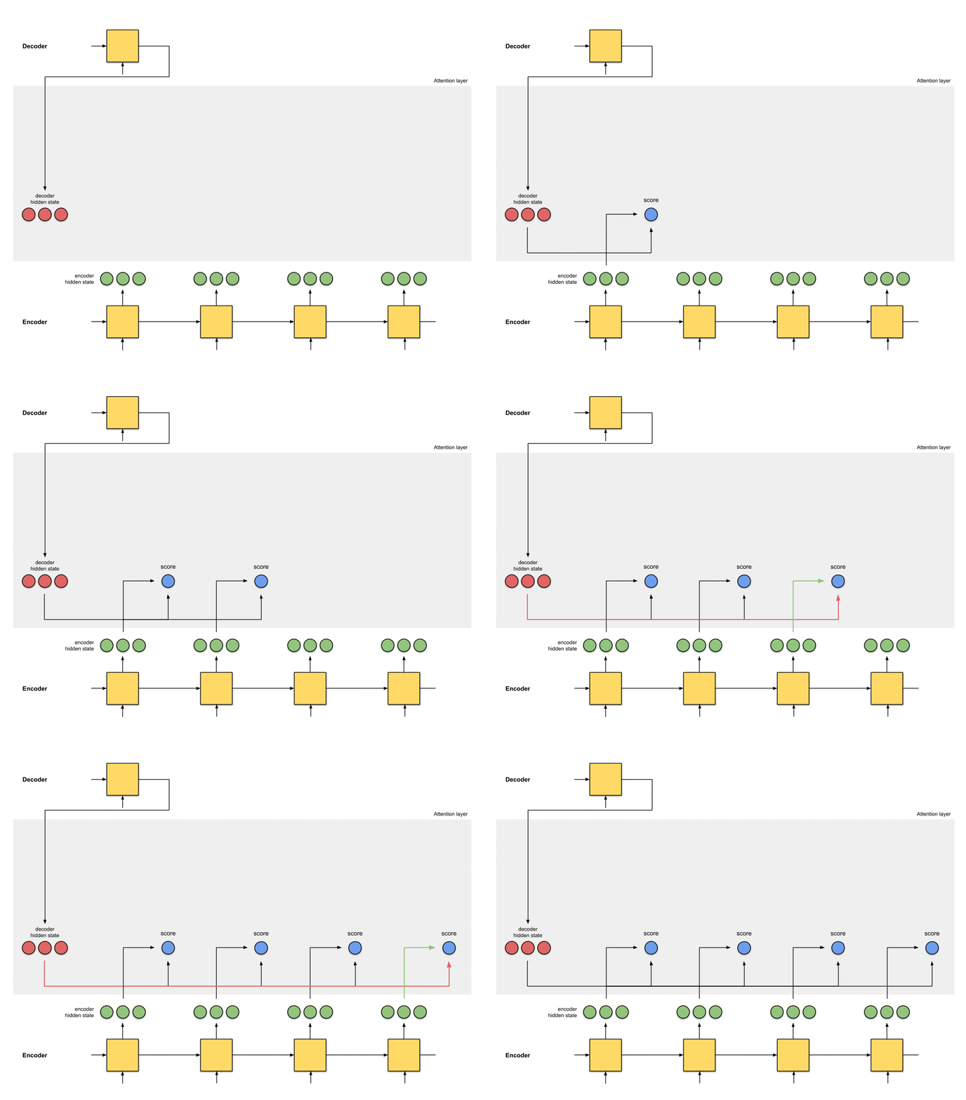
Fig. 1.1: Get the scores
decoder_hidden = [10, 5, 10]
encoder_hidden  score
---------------------
     [0, 1, 1]     15 (= 10×0 + 5×1 + 10×1, the dot product)
     [5, 0, 1]     60
     [1, 1, 0]     15
     [0, 5, 1]     35
在上面的例子当中,编码器隐状态[5,0,1]的attention score最高。这就说明要接下来要被翻译的单词受这个编码器隐状态影响很大。
第三步:把所有的分数进行softmax
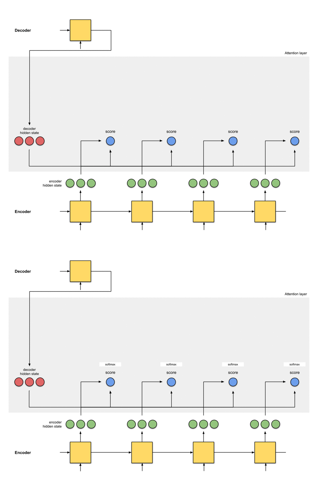
把上一步得到的分数进行softmax处理,变成[0, 1]之间的数,这些被softmax过后的分数表示注意力分布(attention distribution)。
encoder_hidden  score  score^
-----------------------------
     [0, 1, 1]     15       0
     [5, 0, 1]     60       1
     [1, 1, 0]     15       0
     [0, 5, 1]     35       0
注意:上面例子中,分数经过softmax之后变成了[0, 1, 0 ,0],所有的注意力都集中在到了[5, 0, 1]这个隐状态上。在实际操作中,注意力分布的元素并不是非0即1,而是介于0~1之间的浮点数,例如[0.23, 0.53, 0.17, 0.07]
第四步:把每个编码器隐状态和对应的注意力分布相乘
通过把每个编码器隐状态和对应的注意力分布相乘,我们得到了对齐向量(alignment vector 或者叫 annotation vector)。这就是对齐的机制。

Fig. 1.3: Get the alignment vectors`
encoder  score  score^  alignment
---------------------------------
[0, 1, 1]   15      0   [0, 0, 0]
[5, 0, 1]   60      1   [5, 0, 1]
[1, 1, 0]   15      0   [0, 0, 0]
[0, 5, 1]   35      0   [0, 0, 0]
在这我们看到,除了[5,0,1]之外跟所有的编码器隐状态之间的对齐都是[0, 0, 0]。这就说明我们期望第一个翻译的单词要和[5, 0, 1]这个隐状态要匹配起来。
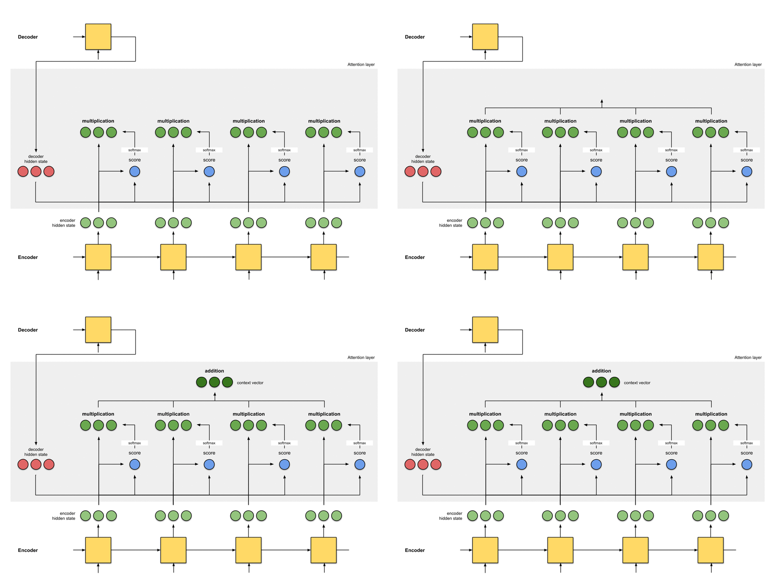
第五步:对齐向量求和
将对齐向量求和,得到context vector。context vector就是上一步计算得到的对齐向量加和之后的整体信息。
encoder   score  score^   alignment
---------------------------------
[0, 1, 1]   15     0     [0, 0, 0]
[5, 0, 1]   60     1     [5, 0, 1]
[1, 1, 0]   15     0     [0, 0, 0]
[0, 5, 1]   35     0     [0, 0, 0]
context = [0+5+0+0, 0+0+0+0, 0+1+0+0] = [5, 0, 1]
第六步:把context vector输入到解码器中
这部分具体的做法取决于网络架构设计,下面介绍三种context vector输入到解码器中的方式,详情见附录B。

写到这里,基本上已经写清楚了,下面给出整个过程的动图。

训练和推断
- 在推断过程中,解码器每一个时刻T的输入是解码器前一个时刻T-1的预测输出。
- 在训练过程中,解码器每一个时刻T的输入是解码器前一个时刻T-1的真实输出
附录A
score function
下面介绍几种分数函数,Additive/concat和dot production上面已经提到了。对于点积操作(比如说点积,余弦相似度等)这类分数函数,其背后的思想就是衡量两个向量之间的相似度。对于前馈神经网络分数函数,其背后思想就是让模型和翻译一同学习到对齐权重。

总结:
| Name | Alignment score function | Citation |
|---|---|---|
| content-base attention | score ( s t , h i ) = cosine [ s t , h i ] \text{score}(\boldsymbol{s}_t, \boldsymbol{h}_i) = \text{cosine}[\boldsymbol{s}_t, \boldsymbol{h}_i] score(st,hi)=cosine[st,hi] | Graves2014 |
| Additive | score ( s t , h i ) = v a ⊤ tanh ( W a [ s t ; h i ] ) \text{score}(\boldsymbol{s}_t, \boldsymbol{h}_i) = \mathbf{v}_a^\top \tanh(\mathbf{W}_a[\boldsymbol{s}_t; \boldsymbol{h}_i]) score(st,hi)=va⊤tanh(Wa[st;hi]) | Bahdanau2015 |
| location-base | α t , i = softmax ( W a s t ) \alpha_{t,i} = \text{softmax}(\mathbf{W}_a \boldsymbol{s}_t) αt,i=softmax(Wast) | Luong2015 |
| General | score ( s t , h i ) = s t ⊤ W a h i \text{score}(\boldsymbol{s}_t, \boldsymbol{h}_i) = \boldsymbol{s}_t^\top\mathbf{W}_a\boldsymbol{h}_i score(st,hi)=st⊤Wahi | Luong2015 |
| dot product | score ( s t , h i ) = s t ⊤ h i \text{score}(\boldsymbol{s}_t, \boldsymbol{h}_i) = \boldsymbol{s}_t^\top\boldsymbol{h}_i score(st,hi)=st⊤hi | Luong2015 |
| scaled dot-product | score ( s t , h i ) = s t ⊤ h i n \text{score}(\boldsymbol{s}_t, \boldsymbol{h}_i) = \frac{\boldsymbol{s}_t^\top\boldsymbol{h}_i}{\sqrt{n}} score(st,hi)=nst⊤hi | Vaswani2017 |
备注:
- Referred to as “concat” in Luong, et al., 2015 and as “additive attention” in Vaswani, et al., 2017
- It adds a scaling factor 1 / n 1/\sqrt{n} 1/n, motivated by the concern when the input is large, the softmax function may have an extremely small gradient, hard for efficient learning
附录B. Attention: Examples
We have seen the both the seq2seq and the seq2seq+attention architectures in the previous section. In the next sub-sections, let’s examine 3 more seq2seq-based architectures for NMT that implement attention. For completeness, I have also appended their Bilingual Evaluation Understudy (BLEU) scores — a standard metric for evaluating a generated sentence to a reference sentence.
2a. Bahdanau et. al (2015) [1]
This implementation of attention is one of the founding attention fathers. The authors use the word ‘align’ in the title of the paper “Neural Machine Translation by Learning to Jointly Align and Translate” to mean adjusting the weights that are directly responsible for the score, while training the model. The following are things to take note about the architecture:
- The encoder is a bidirectional (forward+backward) gated recurrent unit (BiGRU). The decoder is a GRU whose initial hidden state is a vector modified from the last hidden state from the backward encoder GRU (not shown in the diagram below).
- The score function in the attention layer is the additive/concat.
- The input to the next decoder step is the concatenation between the generated word from the previous decoder time step (pink) and context vector from the current time step (dark green).

Fig. 2a: NMT from Bahdanau et. al. Encoder is a BiGRU, decoder is a GRU.
The authors achieved a BLEU score of 26.75 on the WMT’14 English-to-French dataset.
Intuition: seq2seq with bidirectional encoder + attention
Translator A reads the German text while writing down the keywords. Translator B (who takes on a senior role because he has an extra ability to translate a sentence from reading it backwards) reads the same German text from the last word to the first, while jotting down the keywords. These two regularly discuss about every word they read thus far. Once done reading this German text, Translator B is then tasked to translate the German sentence to English word by word, based on the discussion and the consolidated keywords that the both of them have picked up.
Translator A is the forward RNN, Translator B is the backward RNN.
2b. Luong et. al (2015) [2]
The authors of Effective Approaches to Attention-based Neural Machine Translation have made it a point to simplify and generalise the architecture from Bahdanau et. al. Here’s how:
1. The encoder is a two-stacked long short-term memory (LSTM) network. The decoder also has the same architecture, whose initial hidden states are the last encoder hidden states.
2. The score functions they experimented were (i) additive/concat, (ii) dot product, (iii) location-based, and (iv) ‘general’.
3. The concatenation between output from current decoder time step, and context vector from the current time step are fed into a feed-forward neural network to give the final output (pink) of the current decoder time step.

Fig. 2b: NMT from Luong et. al. Encoder is a 2 layer LSTM, likewise for decoder.
On the WMT’15 English-to-German, the model achieved a BLEU score of 25.9.
Intuition: seq2seq with 2-layer stacked encoder + attention
Translator A reads the German text while writing down the keywords. Likewise, Translator B (who is more senior than Translator A) also reads the same German text, while jotting down the keywords. Note that the junior Translator A has to report to Translator B at every word they read. Once done reading, the both of them translate the sentence to English together word by word, based on the consolidated keywords that they have picked up.
2c. Google’s Neural Machine Translation (GNMT) [9]
Because most of us must have used Google Translate in one way or another, I feel that it is imperative to talk about Google’s NMT, which was implemented in 2016. GNMT is a combination of the previous 2 examples we have seen (heavily inspired by the first [1]).
- The encoder consists of a stack of 8 LSTMs, where the first is bidirectional (whose outputs are concatenated), and a residual connection exists between outputs from consecutive layers (starting from the 3rd layer). The decoder is a separate stack of 8 unidirectional LSTMs.
- The score function used is the additive/concat, like in [1].
- Again, like in [1], the input to the next decoder step is the concatenation between the output from the previous decoder time step (pink) and context vector from the current time step (dark green).

Fig. 2c: Google’s NMT for Google Translate. Skip connections are denoted by curved arrows. *Note that the LSTM cells only show the hidden state and input; it does not show the cell state input.
The model achieves 38.95 BLEU on WMT’14 English-to-French, and 24.17 BLEU on WMT’14 English-to-German.
Intuition: GNMT — seq2seq with 8-stacked encoder (+bidirection+residual connections) + attention
8 translators sit in a column from bottom to top, starting with Translator A, B, …, H. Every translator reads the same German text. At every word, Translator A shares his/her findings with Translator B, who will improve it and share it with Translator C — repeat this process until we reach Translator H. Also, while reading the German text, Translator H writes down the relevant keywords based on what he knows and the information he has received.
Once everyone is done reading this English text, Translator A is told to translate the first word. First, he tries to recall, then he shares his answer with Translator B, who improves the answer and shares with Translator C — repeat this until we reach Translator H. Translator H then writes the first translation word, based on the keywords he wrote and the answers he got. Repeat this until we get the translation out.
