【计算机视觉OpenCV基础】实验四 尺寸测量

实验四 尺寸测量

计算机视觉OpenCV基础实验合辑（实验1234+扩展）
资源下载地址： https://download.csdn.net/download/weixin_53403301
合辑：（加在下载地址后面）
/87113581
讲义（包括理论、图例、PPT、实验、代码、手册）：（加在下载地址后面）
/87113633

matplotlib中载入中文字体

plt.rcParams['font.sans-serif'] = ['SimHei'] # 载入字体

实验目的：
1、 通过已知尺寸的首目标来对比测量其他目标尺寸。
2、 标记所有目标尺寸。
实验内容：
1、首目标处理
图像目标尺寸检测类似于计算从我们的相机到一个物体的距离——在这两种情况下，我们都需要事先定义一个比率来测量每个给定度量单位的像素数（pixels_per_metric）。在这里所说的这个被称为“pixels_per_metric”的比率指标，我在接下来的部分中对其更正式的定义。

为了确定图像中物体的大小，我们首先需要使用一个参照物作为“校准”点。我们的参照物应该有两个重要的属性：

1、我们应该知道这个物体的真实尺寸（在宽度或高度上的毫米或英寸等值的大小）。

2、我们应该能够轻松地在图片中找到这个参照物，要么基于参照物的位置(如，参照物可以是一副图像中左上角的物体)或基于参照物的外表(例如参照物可以是图片中具有最独特的颜色或独一无二的形状，不同于所有其他的物体)。一句话而言：在任何一种情况下，我们的参照物都应该是以某种方式进行唯一可识别的The One。

在图中，我们将使用美分硬币作为我们的参照物，其选择方式为选择图像中最左侧的物体作为参照物。

我们将使用一个美分硬币作为我们的参照物，并确保它总是被放置在图像中最左边，这使得我们可以通过对它们位置的轮廓大小进行排序，进一步来提取信息。

通过保证这个美分硬币是最左边的物体后，我们可以从左到右对我们的物体等高线区域进行排列，抓住这个硬币（它将始终对应于排序列表中的第一个等高线区域），并使用它来定义我们的pixels_per_metric比率，我们将其定义为：

pixels_per_metric = 物体像素宽 / 物体真实宽

美分硬币的真实宽度是0.955英寸。现在，假设我们图像中硬币的像素宽为150像素（基于它的相关边界框）。那么这种情况下pixels_per_metric这样计算：

pixels_per_metric = 150px / 0.955in = 157px

因此，在我们这幅图像中，每英寸大约有157个像素。有了这个比率，我们可以计算图像中其他物体的大小了。

1、测量物体大小
既然我们已经理解了pixels_per_metric，我们就可以实现用于测量图像中对象大小的Python程序脚本了。

打开一个新的py文件，插入以下代码：

# -*- coding: utf-8 -*-
"""
Created on Sat May  8 14:19:04 2021
​
@author: ZHOU
"""
​
# 导入库
from scipy.spatial import distance as dist
# from imutils import perspective
# from imutils import contours
import contours
import perspective
import numpy as np
# import argparse
import imutils
import cv2
​
import matplotlib.pyplot as plt
plt.rcParams['font.sans-serif'] = ['SimHei'] # 载入字体
​
​
# card=input('输入图像路径和文件名：')
​
def midpoint(ptA, ptB):
    return ((ptA[0] + ptB[0]) * 0.5, (ptA[1] + ptB[1]) * 0.5)
    
def pshow(words,picture):
    plt.imshow(picture[:,:,::-1])
    plt.title(words), plt.xticks([]), plt.yticks([])
    plt.show()

定义了一个midpoint函数，顾名思义，它用于计算两个（x，y）坐标之间的中点。

然后我们在第14-19行中解析我们的命令行参数。我们需要两个参数，–image，它是我们输入图像的路径，其中包含我们想要测量的对象，–width，也就是我们的参照物的宽度（英寸），–image路径图像中所认定的那个最左边的物体。

我们现在可以加载我们的图像并对其进行预处理：

# 图像导入，预处理
#image = cv2.imread(card)
image = cv2.imread('exp02.png')
​
pshow('原图',image)
gray = cv2.cvtColor(image, cv2.COLOR_BGR2GRAY)
gray = cv2.GaussianBlur(gray, (7, 7), 0)
​
# 执行边缘检测，然后执行膨胀+腐蚀
# 闭合对象边之间的间隙
edged = cv2.Canny(gray, 50, 100)
edged = cv2.dilate(edged, None, iterations=1)
edged = cv2.erode(edged, None, iterations=1)
​
# 在边缘图中查找等高线
#编译器所装cv版本为4.4.0版本，不同版本cv2.findContours语句输出的值的数量、顺序不一样，根据不同版本需进行调整
​
#cv版本4
cnts,a = cv2.findContours(edged.copy(), cv2.RETR_EXTERNAL, cv2.CHAIN_APPROX_SIMPLE)
​
#cv版本3
# a,cnts,b = cv2.findContours(edged.copy(), cv2.RETR_EXTERNAL, cv2.CHAIN_APPROX_SIMPLE) 
​
#cv版本2
# a,cnts = cv2.findContours(edged.copy(), cv2.RETR_EXTERNAL, cv2.CHAIN_APPROX_SIMPLE) 
​
# cnts = cnts[0] if imutils.is_cv2() else cnts[1]
​
# 从左到右排列轮廓并初始化
#“每公制像素”校准变量
(cnts, _) = contours.sort_contours(cnts)
pixelsPerMetric = None

从磁盘加载我们的图像，将其转换为灰度，然后使用高斯过滤器平滑它。然后我们执行边缘检测和扩张+磨平，以消除边缘图中边缘之间的任何间隙。

找到等高线，也就是我们边缘图中物体相对应的轮廓线。

然后，这些等高线区域从左到右（使得我们可以提取到参照物）在第39行中进行排列。然后我们在第40行时，对pixelsPerMetric值进行初始化。

下一步是对每一个等高线区域值大小进行检查校验。

# 分别在轮廓上循环
for c in cnts:
    print(cv2.contourArea(c))
    # 如果轮廓不够大，请忽略它
    if cv2.contourArea(c) < 100:
        continue
    
    # 计算轮廓的旋转边界框
    orig = image.copy()
    box = cv2.minAreaRect(c)
    box = cv2.cv.BoxPoints(box) if imutils.is_cv2() else cv2.boxPoints(box)
    box = np.array(box, dtype="int")
    
    # 对等高线中的点进行排序，使其出现
​
    #在左上角、右上角、右下角和左下角
​
    #顺序，然后绘制旋转边界的轮廓
​
    box = perspective.order_points(box)
    cv2.drawContours(orig, [box.astype("int")], -1, (0, 255, 0), 2)
​
    # 在原始点上循环并绘制它们
    for (x, y) in box:
        cv2.circle(orig, (int(x), int(y)), 5, (0, 0, 255), -1)

开始对每个单独的轮廓值进行循环。如果等高线区域大小不够大，我们就会丢弃该区域，认为它是边缘检测过程遗留下来的噪音。

然后我们将旋转的边界框坐标按顺序排列在左上角，右上角，右下角，左下角。

最后，用绿色画出物体的轮廓，然后将边界框矩形的顶点画在小的红色圆圈中。现在我们已经有了边界框，接下来就可以计算出一系列的中点：

# 打开顺序边界框，然后计算中点
​
#在左上和右上坐标之间，然后
​
#左下角和右下角坐标之间的中点
    (tl, tr, br, bl) = box
    (tltrX, tltrY) = midpoint(tl, tr)
    (blbrX, blbrY) = midpoint(bl, br)
​
    #计算左上角点和右上角点之间的中点，
​
    #然后是右上角和右下角之间的中点
    (tlblX, tlblY) = midpoint(tl, bl)
    (trbrX, trbrY) = midpoint(tr, br)
​
    # 在图像上画中点
    cv2.circle(orig, (int(tltrX), int(tltrY)), 5, (255, 0, 0), -1)
    cv2.circle(orig, (int(blbrX), int(blbrY)), 5, (255, 0, 0), -1)
    cv2.circle(orig, (int(tlblX), int(tlblY)), 5, (255, 0, 0), -1)
    cv2.circle(orig, (int(trbrX), int(trbrY)), 5, (255, 0, 0), -1)
​
    # 在中点之间画线
    cv2.line(orig, (int(tltrX), int(tltrY)), (int(blbrX), int(blbrY)),
        (255, 0, 255), 2)
    cv2.line(orig, (int(tlblX), int(tlblY)), (int(trbrX), int(trbrY)),
        (255, 0, 255), 2)

将我们前面所得的有序边界框各个值拆分出来，然后计算左上角和右上角之间的中点，然后是计算左下角和右下角之间的中点。

此外，我们还分别计算左上角与左下角，右上角和右下角的中点。

在我们的图像上画出蓝色的中点，然后将各中间点用紫色线连接起来。

接下来，我们需要通过查看我们的参照物来初始化pixelsPerMetric变量

    # 计算中点之间的欧氏距离
    dA = dist.euclidean((tltrX, tltrY), (blbrX, blbrY))
    dB = dist.euclidean((tlblX, tlblY), (trbrX, trbrY))
​
    # 如果每个度量的像素尚未初始化，则
​
    #将其计算为像素与所提供度量的比率
​
    #（在本例中，单位为英寸）
    if pixelsPerMetric is None:
        pixelsPerMetric = dB / 24.26 # 输入width
    首先，我们计算中间点集之间的欧几里得距离（第90行和第91行）。
    
    dA变量将包含高度距离（以像素为单位），而dB将保持我们的宽度距离。
    
    然后，我们在第96行进行检查，看看我们的pixelsPerMetric变量是否已经被初始化了，
    
    如果没有，我们将dB除以我们提供的宽度，从而得到每英寸的（近似）像素。
    
    现在我们已经定义了pixelsPerMetric变量，我们可以测量图像中各物体的大小：
  # 计算对象的大小
    dimA = dA / pixelsPerMetric
    dimB = dB / pixelsPerMetric
​
    # 在图像上绘制对象大小
    cv2.putText(orig, "{:.1f}in".format(dimA),
        (int(tltrX - 15), int(tltrY - 10)), cv2.FONT_HERSHEY_SIMPLEX,
        0.65, (255, 255, 255), 2)
    cv2.putText(orig, "{:.1f}in".format(dimB),
        (int(trbrX + 10), int(trbrY)), cv2.FONT_HERSHEY_SIMPLEX,
        0.65, (255, 255, 255), 2)
​
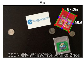
    # 显示结果
    pshow('结果',orig)

计算物体的尺寸（英寸），方法是通过pixelsper度量值划分各自的欧几里得距离。 在我们的图像上画出物体的尺寸，而后显示输出结果。

总代码：

# -*- coding: utf-8 -*-
"""
Created on Sat May  8 14:19:04 2021

@author: ZHOU
"""

# import the necessary packages
from scipy.spatial import distance as dist
# from imutils import perspective
# from imutils import contours
import contours
import perspective
import numpy as np
# import argparse
import imutils
import cv2

import matplotlib.pyplot as plt
plt.rcParams['font.sans-serif'] = ['SimHei'] # 载入字体

card=input('输入图像路径和文件名：')

def midpoint(ptA, ptB):
    return ((ptA[0] + ptB[0]) * 0.5, (ptA[1] + ptB[1]) * 0.5)
    
def pshow(words,picture):
    plt.imshow(picture[:,:,::-1])
    plt.title(words), plt.xticks([]), plt.yticks([])
    plt.show()
    
# load the image, convert it to grayscale, and blur it slightly
image = cv2.imread(card)
pshow('原图',image)
gray = cv2.cvtColor(image, cv2.COLOR_BGR2GRAY)
gray = cv2.GaussianBlur(gray, (7, 7), 0)

# perform edge detection, then perform a dilation + erosion to
# close gaps in between object edges
edged = cv2.Canny(gray, 50, 100)
edged = cv2.dilate(edged, None, iterations=1)
edged = cv2.erode(edged, None, iterations=1)

# find contours in the edge map
cnts,a = cv2.findContours(edged.copy(), cv2.RETR_EXTERNAL, cv2.CHAIN_APPROX_SIMPLE)
# cnts = cnts[0] if imutils.is_cv2() else cnts[1]

# sort the contours from left-to-right and initialize the
# 'pixels per metric' calibration variable
(cnts, _) = contours.sort_contours(cnts)
pixelsPerMetric = None

# loop over the contours individually
for c in cnts:
    print(cv2.contourArea(c))
    # if the contour is not sufficiently large, ignore it
    if cv2.contourArea(c) < 100:
        continue
    
    # compute the rotated bounding box of the contour
    orig = image.copy()
    box = cv2.minAreaRect(c)
    box = cv2.cv.BoxPoints(box) if imutils.is_cv2() else cv2.boxPoints(box)
    box = np.array(box, dtype="int")
    
    # order the points in the contour such that they appear
    # in top-left, top-right, bottom-right, and bottom-left
    # order, then draw the outline of the rotated bounding
    # box
    box = perspective.order_points(box)
    cv2.drawContours(orig, [box.astype("int")], -1, (0, 255, 0), 2)

    # loop over the original points and draw them
    for (x, y) in box:
        cv2.circle(orig, (int(x), int(y)), 5, (0, 0, 255), -1)
        
    # unpack the ordered bounding box, then compute the midpoint
    # between the top-left and top-right coordinates, followed by
    # the midpoint between bottom-left and bottom-right coordinates
    (tl, tr, br, bl) = box
    (tltrX, tltrY) = midpoint(tl, tr)
    (blbrX, blbrY) = midpoint(bl, br)

    # compute the midpoint between the top-left and top-right points,
    # followed by the midpoint between the top-righ and bottom-right
    (tlblX, tlblY) = midpoint(tl, bl)
    (trbrX, trbrY) = midpoint(tr, br)

    # draw the midpoints on the image
    cv2.circle(orig, (int(tltrX), int(tltrY)), 5, (255, 0, 0), -1)
    cv2.circle(orig, (int(blbrX), int(blbrY)), 5, (255, 0, 0), -1)
    cv2.circle(orig, (int(tlblX), int(tlblY)), 5, (255, 0, 0), -1)
    cv2.circle(orig, (int(trbrX), int(trbrY)), 5, (255, 0, 0), -1)

    # draw lines between the midpoints
    cv2.line(orig, (int(tltrX), int(tltrY)), (int(blbrX), int(blbrY)),
        (255, 0, 255), 2)
    cv2.line(orig, (int(tlblX), int(tlblY)), (int(trbrX), int(trbrY)),
        (255, 0, 255), 2)
    
    # compute the Euclidean distance between the midpoints
    dA = dist.euclidean((tltrX, tltrY), (blbrX, blbrY))
    dB = dist.euclidean((tlblX, tlblY), (trbrX, trbrY))

    # if the pixels per metric has not been initialized, then
    # compute it as the ratio of pixels to supplied metric
    # (in this case, inches)
    if pixelsPerMetric is None:
        pixelsPerMetric = dB / 24.26 # args["width"]

    # compute the size of the object
    dimA = dA / pixelsPerMetric
    dimB = dB / pixelsPerMetric

    # draw the object sizes on the image
    cv2.putText(orig, "{:.1f}in".format(dimA),
        (int(tltrX - 15), int(tltrY - 10)), cv2.FONT_HERSHEY_SIMPLEX,
        0.65, (255, 255, 255), 2)
    cv2.putText(orig, "{:.1f}in".format(dimB),
        (int(trbrX + 10), int(trbrY)), cv2.FONT_HERSHEY_SIMPLEX,
        0.65, (255, 255, 255), 2)

    # show the output image
    pshow('结果',orig)

    

输入图像路径和文件名：./exp01.png

1032.0

10137.0

1035.5

8281.5

8755.5

804.5

实验收获：
学会了利用OpenCV通过已知尺寸的首目标来对比测量其他目标尺寸并标记所有目标尺寸，成功在不同的目标上进行匹配和标注。