LoG 和 DoG的本质联系与区别
1.Laplacian/Laplacian of Gaussian1 (LoG)
As Laplace operator may detect edges as well as noise (isolated, out-of-range), it may be desirable to smooth the image first by a convolution with a Gaussian kernel of width 

to suppress the noise before using Laplace for edge detection:
![\begin{displaymath}\bigtriangleup[G_{\sigma}(x,y) * f(x,y)]=[\bigtriangleup G_{\sigma}(x,y)] * f(x,y)=LoG*f(x,y)\end{displaymath}](http://img.e-com-net.com/image/info8/fe61636a5f0f4ea29c8391ad029ed33d.png)
The first equal sign is due to the fact that
![\begin{displaymath}\frac{d}{dt}[h(t)*f(t)]=\frac{d}{dt} \int f(\tau) h(t-\tau)d\......int f(\tau) \frac{d}{dt} h(t-\tau)d\tau=f(t)*\frac{d}{dt} h(t)\end{displaymath}](http://img.e-com-net.com/image/info8/874d81d613fd4ff282a7c109fae25ec8.png)
So we can obtain the Laplacian of Gaussian
 first and then convolve it with the input image. To do so, first consider
and

Note that for simplicity we omitted the normalizing coefficient
 . Similarly we can get
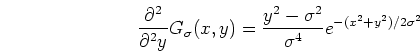
Now we have LoG as an operator or convolution kernel defined as

The Gaussian  and its first and second derivatives
  and
and  are shown here:


This 2-D LoG can be approximated by a 5 by 5 convolution kernel such as
![\begin{displaymath}\left[ \begin{array}{ccccc}0 & 0 & 1 & 0 & 0 \\0 & 1 &......0 & 1 & 2 & 1 & 0 \\0 & 0 & 1 & 0 & 0 \end{array} \right]\end{displaymath}](http://img.e-com-net.com/image/info8/ffa4f5665d2842fd81aa525cac62f27b.png)
The kernel of any other sizes can be obtained by approximating the continuous expression of LoG given above. However, make sure that the sum (or average) of all elements of the kernel has to be zero (similar to the Laplace kernel) so that the convolution result of a homogeneous regions is always zero.
The edges in the image can be obtained by these steps:
- Applying LoG to the image
- Detection of zero-crossings in the image
- Threshold the zero-crossings to keep only those strong ones (large difference between the positive maximum and the negative minimum)

2.Difference of Gaussian (DoG)
Similar to Laplace of Gaussian, the image is first smoothed by convolution with Gaussian kernel of certain width
to get
With a different width , a second smoothed image can be obtained:
We can show that the difference of these two Gaussian smoothed images, called difference of Gaussian (DoG), can be used to detect edges in the image.
The DoG as an operator or convolution kernel is defined as
Both 1-D and 2-D functions of and and their difference are shown below:
As the difference between two differently low-pass filtered images, the DoG is actually a band-pass filter, which removes high frequency components representing noise, and also some low frequency components representing the homogeneous areas in the image. The frequency components in the passing band are assumed to be associated to the edges in the images.
The discrete convolution kernel for DoG can be obtained by approximating the continuous expression of DoG given above. Again, it is necessary for the sum or average of all elements of the kernel matrix to be zero.
Comparing this plot with the previous one, we see that the DoG curve is very similar to the LoG curve. Also, similar to the case of LoG, the edges in the image can be obtained by these steps:
- Applying DoG to the image
- Detection of zero-crossings in the image
- Threshold the zero-crossings to keep only those strong ones (large difference between the positive maximum and the negative minimum)
Edge detection by DoG operator:
讲义的地址:http://fourier.eng.hmc.edu/e161/lectures/gradient/gradient.html
基础知识:
1.1Gradient
The Gradient (also called the Hamilton operator) is a vector operator for any N-dimensional scalar function , where is an N-D vector variable. For example, when , may represent temperature, concentration, or pressure in the 3-D space. The gradient of this N-D function is a vector composed of components for the partial derivatives:
- The direction of the gradient vector is the direction in the N-D space along which the function increases most rapidly.
- The magnitude of the gradient is the rate of the increment.
In image processing we only consider 2-D field:
When applied to a 2-D function , this operator produces a vector function:
where and . The direction and magnitude of are respectively
Now we show that increases most rapidly along the direction of and the rate of increment is equal to the magnitude of .
Consider the directional derivative of along an arbitrary direction :
This directional derivative is a function of , defined as the angle between directions and the positive direction of . To find the direction along which is maximized, we let
Solving this for , we get
i.e.,
which is indeed the direction of .
From , we can also get
Substituting these into the expression of , we obtain its maximum magnitude,
which is the magnitude of .
For discrete digital images, the derivative in gradient operation
becomes the difference
Two steps for finding discrete gradient of a digital image:
- Find the difference: in the two directions:
- Find the magnitude and direction of the gradient vector:
The differences in two directions and can be obtained by convolution with the following kernels:
- Roberts
or
- Sobel (3x3)
- Prewitt (3x3)
- Prewitt (4x4)
The Laplace operator is a scalar operator defined as the dot product (inner product) of two gradient vector operators:
In dimensional space, we have:
When applied to a 2-D function , this operator produces a scalar function:
In discrete case, the second order differentiation becomes second order difference. In 1-D case, if the first order difference is defined as
then the second order difference is
![$\displaystyle \bigtriangleup f[n]$](http://img.e-com-net.com/image/info8/d13d97d334994861a756dd179a1e30e0.png) |
 |
![$\displaystyle \bigtriangledown^2 f[n]=f''[n]=D^2_n[f[n]]=f'[n]-f'[n-1]$](http://img.e-com-net.com/image/info8/095f184f89e4417b8c38159d7bd106ca.png) |
|
|
![$\displaystyle (f[n+1]-f[n])-(f[n]-f[n-1])=f[n+1]-2f[n]+f[n-1]$](http://img.e-com-net.com/image/info8/7e5eb81b9e9244dba9db0ab7a629f062.png) |
Note that
![$f''[n]$](http://img.e-com-net.com/image/info8/d9a205ea52284ecca9e5df411360460e.png) is so defined that it is symmetric to the center element
is so defined that it is symmetric to the center element
![$f[n]$](http://img.e-com-net.com/image/info8/13ced942c3744323b68d485e576b4551.png) . The Laplace operation can be carried out by 1-D convolution with a kernel
. The Laplace operation can be carried out by 1-D convolution with a kernel
![$[1, -2, 1]$](http://img.e-com-net.com/image/info8/b24e5d1190b74ec2ad08e81a5dc0097c.png) .
.
In 2-D case, Laplace operator is the sum of two second order differences in both dimensions:
![$\displaystyle \bigtriangleup f[m,n]$](http://img.e-com-net.com/image/info8/f27d607025ef4cdaab4c8e1ce0a33b37.png) |
|
![$\displaystyle D^2_m[f[m,n]]+D^2_n[f[m,n]]$](http://img.e-com-net.com/image/info8/b445093dfe41469d9be69e743b8d8774.png) |
|
|
![$\displaystyle f[m+1,n]-2f[m,n]+f[m-1,n]+f[m,n+1]-2f[m,n]+f[m,n-1]$](http://img.e-com-net.com/image/info8/d5346c5840fc4103890e8903608ed2ff.png) |
||
|
![$\displaystyle f[m+1,n]+f[m-1,n]+f[m,n+1]+f[m,n-1]-4f[m,n]$](http://img.e-com-net.com/image/info8/de3fc82b433249ffa5da62d9a0f1e0a6.png) |
This operation can be carried out by 2-D convolution kernel:
![\begin{displaymath}\left[ \begin{array}{ccc} 0 & 1 & 0 1 & -4 & 1 0 & 1 & 0\end{array} \right] \end{displaymath}](http://img.e-com-net.com/image/info8/4ac9910266ea46919bd575149fab7f2c.png)
Other Laplace kernels can be used:
![\begin{displaymath}\left[ \begin{array}{ccc} 1 & 1 & 1 1 & -8 & 1 1 & 1 & 1\end{array} \right] \end{displaymath}](http://img.e-com-net.com/image/info8/32d7f9caf0f443ce9781be7daa1794ec.png)
We see that these Laplace kernels are actually the same as the high-pass filtering kernels discussed before.
Gradient operation is an effective detector for sharp edges where the pixel gray levels change over space very rapidly. But when the gray levels change slowly from dark to bright (red in the figure below), the gradient operation will produce a very wide edge (green in the figure). It is helpful in this case to consider using the Laplace operation. The second order derivative of the wide edge (blue in the figure) will have a zero crossing in the middle of edge. Therefore the location of the edge can be obtained by detecting the zero-crossings of the second order difference of the image.
One dimensional example:
In the two dimensional example, the image is on the left, the two Laplace kernels generate two similar results with zero-crossings on the right:
Edge detection by Laplace operator followed by zero-crossing detection: