【Pandas】Pandas数据分析题

数据集下载

Chipotle快餐数据

题目如下

– 将数据集存入一个名为chipo的数据框内
– 查看前10行内容
– 数据集中有多少个列(columns)？
– 打印出全部的列名称
– 数据集的索引是怎样的？
– 被下单数最多商品(item)是什么?
– 在item_name这一列中，一共有多少种商品被下单？
– 在choice_description中，下单次数最多的商品是什么？
– 一共有多少商品被下单？
– 将item_price转换为浮点数
– 在该数据集对应的时期内，收入(revenue)是多少？
– 在该数据集对应的时期内，一共有多少订单？
– 每一单(order)对应的平均总价是多少？

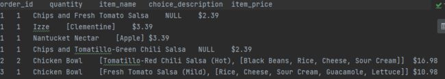
数据前几行展示

# -- 将数据集存入一个名为chipo的数据框内
chipo = pd.read_table('resource/chipotle.tsv', sep='\t', engine='python')

# -- 查看前10行内容
chipo.head(10)

# -- 数据集中有多少个列(columns)？
count_columns = chipo.shape[1]

# -- 打印出全部的列名称
columns = chipo.columns

# -- 数据集的索引是怎样的？
df_index = chipo.index

# -- 被下单数最多商品(item)是什么?
item_max_quantity = chipo[['item_name', 'quantity']].groupby(by=['item_name']).sum().sort_values(by=['quantity'],
                                                                                                 ascending=False).head(
    1)
# -- 在item_name这一列中，一共有多少种商品被下单？
unique_item = chipo.item_name.nunique()
unique_item = chipo['item_name'].nunique()

# -- 在choice_description中，下单次数最多的商品是什么？
choice_description_max = chipo['choice_description'].value_counts().head(1)

# -- 一共有多少商品被下单？
quantity_sum = chipo['quantity'].sum()

# -- 将item_price转换为浮点数
chipo['item_price'] = chipo['item_price'].apply(lambda x: float(x[1:]))

# -- 在该数据集对应的时期内，收入(revenue)是多少？
all_money = (chipo['quantity'] * chipo['item_price']).sum()

# -- 在该数据集对应的时期内，一共有多少订单？
chipo['order_id'].nunique()

# -- 每一单(order)对应的平均总价是多少？
chipo['item_price_sum'] = chipo['quantity'] * chipo['item_price']
(chipo[['order_id', 'item_price_sum']].groupby(by=['order_id']).sum()).mean()

其中apply的应用:
apply函数是pandas里面所有函数中自由度最高的函数。该函数如下：

DataFrame.apply(func, axis=0, broadcast=False, raw=False, reduce=None, args=(), **kwds)

该函数最有用的是第一个参数，这个参数是函数，相当于C/C++的函数指针。

这个函数需要自己实现，函数的传入参数根据axis来定，比如axis = 1，就会把一行数据作为Series的数据 结构传入给自己实现的函数中，我们在函数中实现对Series不同属性之间的计算，返回一个结果，则apply函数 会自动遍历每一行DataFrame的数据，最后将所有结果组合成一个Series数据结构并返回。

数据的过滤和排序(探索2012欧洲杯数据)

数据展示

题目

– 将数据集命名为euro12
– 只选取 Goals 这一列
– 有多少球队参与了2012欧洲杯？
– 该数据集中一共有多少列(columns)?
– 将数据集中的列Team, Yellow Cards和Red Cards单独存为一个名叫discipline的数据框
– 对数据框discipline按照先Red Cards再Yellow Cards进行排序
– 计算每个球队拿到的黄牌数的平均值
– 找到进球数Goals超过6的球队数据
– 选取以字母G开头的球队数据
– 选取前7列
– 选取除了最后3列之外的全部列
– 找到英格兰(England)、意大利(Italy)和俄罗斯(Russia)的射正率(Shooting Accuracy)

# -- 将数据集命名为euro
euro = pd.read_csv('resource/Euro2012.csv')

# -- 只选取 Goals 这一列
Goals = euro['Goals']
Goals = euro.Goals

# -- 有多少球队参与了2012欧洲杯？
item_all = euro['Team'].nunique()

# -- 该数据集中一共有多少列(columns)?
columns_all = euro.shape[1]

# -- 将数据集中的列Team, Yellow Cards和Red Cards单独存为一个名叫discipline的数据框
discipline = euro[['Team', 'Yellow Cards', 'Red Cards']]

# -- 对数据框discipline按照先Red Cards再Yellow Cards进行排序
discipline_sort = discipline.sort_values(['Red Cards', 'Yellow Cards'], ascending=[True, False])

# -- 计算每个球队拿到的黄牌数的平均值
Yellow_Card_Mean = discipline['Yellow Cards'].mean()

# -- 找到进球数Goals超过6的球队数据
Goals_over_six = euro[euro['Goals'] > 6]

# -- 选取以字母G开头的球队数据
Time_Start_With_G = euro[euro['Team'].str.startswith('G')]

# -- 选取前7列
head_seven_columns = euro.iloc[:, :7]

# -- 选取除了最后3列之外的全部列
except_last_three = euro.iloc[:, :-3]

# -- 找到英格兰(England)、意大利(Italy)和俄罗斯(Russia)的射正率(Shooting Accuracy)
data = euro.loc[euro['Team'].isin(['England', 'Italy', 'Russia']), ['Team', 'Shooting Accuracy']]

iloc和loc

• pandas以类似字典的方式来获取某一列的值，比如df['A']，这会得到df的A列，返回的也是一个Series对象。如果想要获取部分行的话就得用到切片

• 例如：df'[:3]，获取前三行；df[3:4]，获取第四行。但是如果想要获取部分行部分列的上述两种方法就无能为力了。这时就得用到ix, loc,iloc方法(ix已弃用)loc是指location的意思，iloc中的i是指integer。iloc和loc方式索引也更为精细。这两者的区别如下：

  loc works on labels in the index # 说白了就是标签索引 
  iloc works on the positions in the index # (so it only takes integers). (位置索引，和列表索引类似，里面只能是数字)
  

跳转顶部

---

探索酒类消费数据

数据展示

题目展示

– 将数据框命名为drinks
– 哪个大陆(continent)平均消耗的啤酒(beer)更多？
– 打印出每个大陆(continent)的红酒消耗(wine_servings)的描述性统计值
– 打印出每个大陆每种酒类别的消耗平均值
– 打印出每个大陆每种酒类别的消耗中位数
– 打印出每个大陆对spirit饮品消耗的平均值，最大值和最小值

# -- 将数据框命名为drinks
drinks = pd.read_csv('resource/drinks.csv')

# -- 哪个大陆(continent)平均消耗的啤酒(beer)更多？
max_beer = drinks[['continent', 'beer_servings']].groupby('continent').mean().sort_values('beer_servings').head(1)

# -- 打印出每个大陆(continent)的红酒消耗(wine_servings)的描述性统计值
continent_wine_des = drinks.groupby('continent')['wine_servings'].describe()

# -- 打印出每个大陆每种酒类别的消耗平均值
continent_mean = drinks.groupby('continent').mean()

# -- 打印出每个大陆每种酒类别的消耗中位数
continent_median = drinks.groupby('continent').median()

# -- 打印出每个大陆对spirit饮品消耗的平均值，最大值和最小值
continent_spirit_des = drinks.groupby('continent').spirit_servings.describe()

跳转顶部

---

探索1960 - 2014 美国犯罪数据

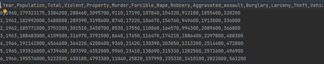
数据展示

题目展示

– 将数据框命名为crime
– 每一列(column)的数据类型是什么样的？
– 将Year的数据类型转换为 datetime64
– 将列Year设置为数据框的索引
– 删除名为Total的列
– 按照Year（每十年）对数据框进行分组并求和
– 何时是美国历史上生存最危险的年代？

# -- 将数据框命名为crime
crime = pd.read_csv('resource/US_Crime_Rates_1960_2014.csv')

# -- 每一列(column)的数据类型是什么样的？
columns_type = crime.info()

# -- 将Year的数据类型转换为 datetime64
crime['Year'] = pd.to_datetime(crime['Year'], format='%Y')

# -- 将列Year设置为数据框的索引
crime = crime.set_index('Year', drop=True)

# -- 删除名为Total的列
del crime['Total']

# -- 按照Year（每十年）对数据框进行分组并求和
crimes = crime.resample('10AS').sum()
population = crime.resample('10AS').max()  # 人口是累计数，不能直接求和
crimes['Population'] = population

# -- 何时是美国历史上生存最危险的年代？
crime.idxmax(0)  # 最大值的索引值

跳转顶部

---

合并–探索虚拟姓名数据

数据是自己创建的

raw_data_1 = {
        'subject_id': ['1', '2', '3', '4', '5'],
        'first_name': ['Alex', 'Amy', 'Allen', 'Alice', 'Ayoung'], 
        'last_name': ['Anderson', 'Ackerman', 'Ali', 'Aoni', 'Atiches']}

raw_data_2 = {
        'subject_id': ['4', '5', '6', '7', '8'],
        'first_name': ['Billy', 'Brian', 'Bran', 'Bryce', 'Betty'], 
        'last_name': ['Bonder', 'Black', 'Balwner', 'Brice', 'Btisan']}

raw_data_3 = {
        'subject_id': ['1', '2', '3', '4', '5', '7', '8', '9', '10', '11'],
        'test_id': [51, 15, 15, 61, 16, 14, 15, 1, 61, 16]}

题目展示

– 创建DataFrame
– 将上述的DataFrame分别命名为data1, data2, data3
– 将data1和data2两个数据框按照行的维度进行合并，命名为all_data
– 将data1和data2两个数据框按照列的维度进行合并，命名为all_data_col
– 打印data3
– 按照subject_id的值对all_data和data3作合并
– 对data1和data2按照subject_id作连接
– 找到 data1 和 data2 合并之后的所有匹配结果

跳转顶部

---

raw_data_1 = {
    'subject_id': ['1', '2', '3', '4', '5'],
    'first_name': ['Alex', 'Amy', 'Allen', 'Alice', 'Ayoung'],
    'last_name': ['Anderson', 'Ackerman', 'Ali', 'Aoni', 'Atiches']}

raw_data_2 = {
    'subject_id': ['4', '5', '6', '7', '8'],
    'first_name': ['Billy', 'Brian', 'Bran', 'Bryce', 'Betty'],
    'last_name': ['Bonder', 'Black', 'Balwner', 'Brice', 'Btisan']}

raw_data_3 = {
    'subject_id': ['1', '2', '3', '4', '5', '7', '8', '9', '10', '11'],
    'test_id': [51, 15, 15, 61, 16, 14, 15, 1, 61, 16]}

# -- 将上述的DataFrame分别命名为data1, data2, data3
data1 = pd.DataFrame(raw_data_1)
data2 = pd.DataFrame(raw_data_2)
data3 = pd.DataFrame(raw_data_3)

# -- 将data1和data2两个数据框按照行的维度进行合并，命名为all_data
all_data = pd.concat([data1, data2], axis=0)

# -- 将data1和data2两个数据框按照列的维度进行合并，命名为all_data_col
all_data_col = pd.concat([data1, data2], axis=1)

# -- 按照subject_id的值对all_data和data3作合并
subject_id_data = pd.merge(all_data, data3, on='subject_id')

# -- 对data1和data2按照subject_id作内连接
inner_join = pd.merge(data1, data2, on='subject_id', how='inner')

# -- 找到 data1 和 data2 合并之后的所有匹配结果
all_join = pd.merge(data1, data2, on='subject_id', how='outer')

统计–探索风速数据

数据展示

题目展示

– 将数据作存储并且设置前三列为合适的索引
– 2061年？我们真的有这一年的数据？创建一个函数并用它去修复这个bug
– 将日期设为索引，注意数据类型，应该是datetime64[ns]
– 对应每一个location，一共有多少数据值缺失
– 对应每一个location，一共有多少完整的数据值
– 对于全体数据，计算风速的平均值
– 创建一个名为loc_stats的数据框去计算并存储每个location的风速最小值，最大值，平均值和标准差
– 创建一个名为day_stats的数据框去计算并存储所有location的风速最小值，最大值，平均值和标准差
– 对于每一个location，计算一月份的平均风速
– 对于数据记录按照年为频率取样
– 对于数据记录按照月为频率取样

# -- 将数据作存储并且设置前三列为合适的索引
wind = pd.read_csv('resource/wind.csv', sep='\s+', parse_dates=[[0, 1, 2]])  # \s+表示任意的空白字符


# -- 2061年？我们真的有这一年的数据？创建一个函数并用它去修复这个bug
def fix_century(x):
    year = x.year - 100 if x.year > 1900 else x.yeaa
    return datetime.date(year, x.month, x.day)


wind['Yr_Mo_Dy'] = wind['Yr_Mo_Dy'].apply(fix_century)

# -- 将日期设为索引，注意数据类型，应该是datetime64[ns]
wind['Yr_Mo_Dy'] = pd.to_datetime(wind['Yr_Mo_Dy'])
wind = wind.set_index('Yr_Mo_Dy')

# -- 对应每一个location，一共有多少数据值缺失
null_count = wind.isnull().sum()

# -- 对应每一个location，一共有多少完整的数据值
not_null_count = wind.shape[1] - wind.isnull().sum()

# -- 对于全体数据，计算风速的平均值
data_mean = wind.mean().mean()

# -- 创建一个名为loc_stats的数据框去计算并存储每个location的风速最小值，最大值，平均值和标准差
loc_stats = pd.DataFrame()
loc_stats['min'] = wind.min()
loc_stats['max'] = wind.max()
loc_stats['mean'] = wind.mean()
loc_stats['std'] = wind.std()

# -- 创建一个名为day_stats的数据框去计算并存储所有location的风速最小值，最大值，平均值和标准差
day_stats = pd.DataFrame()
day_stats['min'] = wind.min(axis=1)
day_stats['max'] = wind.max(axis=1)
day_stats['mean'] = wind.mean(axis=1)
day_stats['std'] = wind.std(axis=1)

# -- 对于每一个location，计算一月份的平均风速
wind['date'] = wind.index

wind['year'] = wind['date'].apply(lambda df: df.year)
wind['month'] = wind['date'].apply(lambda df: df.month)
wind['day'] = wind['date'].apply(lambda df: df.day)
january_winds = wind.query('month ==1')  # query等同于df[df.month==1]
january_winds.loc[:, 'RPT':'MAL'].mean()

# -- 对于数据记录按照年为频率取样
wind.query('month ==1 and day == 1')

# -- 对于数据记录按照月为频率取样
wind.query('day == 1')

跳转顶部

---

时间序列–探索Apple公司股价数据

数据展示

题目展示

– 读取数据并存为一个名叫apple的数据框
– 查看每一列的数据类型
– 将Date这个列转换为datetime类型
– 将Date设置为索引
– 有重复的日期吗？
– 将index设置为升序
– 找到每个月的最后一个交易日(business day)
– 数据集中最早的日期和最晚的日期相差多少天？
– 在数据中一共有多少个月？

# -- 读取数据并存为一个名叫apple的数据框
apple = pd.read_csv('resource/appl_1980_2014.csv')

# -- 查看每一列的数据类型
columns_type = apple.info()

# -- 将Date这个列转换为datetime类型
apple['Date'] = pd.to_datetime(apple['Date'])

# -- 将Date设置为索引
apple = apple.set_index('Date')

# -- 有重复的日期吗？
data = apple.index.is_unique

# -- 将index设置为升序
apple = apple.sort_index(ascending=True)

# -- 找到每个月的最后一个交易日(business day)
apple_month = apple.resample('BM').mean()

# -- 数据集中最早的日期和最晚的日期相差多少天？
max_min = (apple.index.max() - apple.index.min()).days

# -- 在数据中一共有多少个月？
month_sum = apple['Adj Close'].plot(title='Apple Stock').get_figure().set_size_inches(9, 5)

跳转顶部

---

删除–探索Iris纸鸢花数据

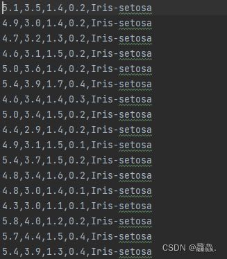
数据展示

题目展示

– 将数据集存成变量iris
– 创建数据框的列名称[‘sepal_length’,‘sepal_width’, ‘petal_length’, ‘petal_width’, ‘class’]
– 数据框中有缺失值吗？
– 将列petal_length的第10到19行设置为缺失值
– 将petal_lengt缺失值全部替换为1.0
– 删除列class
– 将数据框前三行设置为缺失值
– 删除有缺失值的行
– 重新设置索引

# -- 将数据集存成变量iris
iris = pd.read_csv('resource/iris.data', header=None)

# -- 创建数据框的列名称['sepal_length','sepal_width', 'petal_length', 'petal_width', 'class']
iris.columns = ['sepal_length', 'sepal_width', 'petal_length', 'petal_width', 'class']

# -- 数据框中有缺失值吗？
null_sum = iris.isnull().sum()

# -- 将列petal_length的第10到19行设置为缺失值
iris['petal_length'].loc[10:19] = np.nan

# -- 将petal_length缺失值全部替换为1.0
iris['petal_length'].fillna(1, inplace=True)

# -- 删除列class
del iris['class']

# -- 将数据框前三行设置为缺失值
iris.loc[0:2, :] = np.nan

# -- 删除有缺失值的行
iris = iris.dropna(how='any')

# -- 重新设置索引
iris = iris.reset_index(drop=True)  # 加上drop参数，原有索引就不会成为新的列

跳转顶部

---