Stochastic Weight Averaging (SWA) 随机权重平均

最近在参加公司的AI竞赛，刚好用到了Stochastic Weight Averaging的方法，所以也简单看了下提出这个方法的论文Averaging Weights Leads to Wider Optima and Better Generalization，这是一种容易实现、简单、基本没有额外计算开销却能比较可观地提升DNN模型效果的方法，在这里写写自己对这篇论文的一些理解。

相关链接

paper：https://arxiv.org/abs/1803.05407

code：https://github.com/timgaripov/swa

pytorch：https://pytorch.org/blog/pytorch-1.6-now-includes-stochastic-weight-averaging/

基础

Loss Surfaces, Mode Connectivity, and Fast Ensembling of DNNs

swa这篇论文基本上是以上面的论文为基础，而且作者是一样的，是一脉相承的工作，所以上面的论文算是前作，其主要的发现和贡献有以下两点：

• local optima found by SGD can be connected by simple curves of near constant loss（由SGD找到的局部最优解可以被近似恒定损失的简单曲线连接起来，这点很重要，后面可以看到swa其实就是对在这样的区域上探索得到的权重进行平均）

• Fast Geometric Ensembling (FGE，根据上面的发现提出的一种集成方法)

  sample multiple nearby points in weight space to create high performing ensembles in the time required to train a single DNN（这种集成方法的主要思想是在训练单个DNN所需的时间内从权重空间中采样多个相近的点，用于创建高性能的模型集合）

思路

通过研读论文，我猜测其写作的大概思路是这样：

1. FGE洞察train loss和test error几何平面，发现对FGE采样的模型的权重进行平均可以得到更好的模型权重

2. 可否直接在SGD过程中得到这些点并进行平均

   We show that SGD with cyclical [e.g., Loshchilov and Hutter, 2017] and constant learning rates traverses regions of weight space corresponding to high-performing networks. We find that while these models are moving around this optimal set they never reach its central points. We show that we can move into this more desirable space of points by averaging the weights proposed over SGD iterations.

   简单地说，使用循环学习率调度或者固定学习率的SGD能够遍历和高性能网络相关联的权重空间区域，但是只是在这个区域周围移动而没有到达中心点。通过对SGD迭代产生的权重进行平均可以解决问题。

3. 同样是较优的集合中的点，为什么靠近中心的点会有更好的泛化性能呢？

   • We demonstrate that SWA leads to solutions that are wider than the optima found by SGD. Keskar et al. [2017] and Hochreiter and Schmidhuber [1997] conjecture that the width of the optima is critically related to generalization. We illustrate that the loss on the train is shifted with respect to the test error. We show that SGD generally converges to a point near the boundary of the wide flat region of optimal points. SWA on the other hand is able to find a point centered in this region, often with slightly worse train loss but with substantially better test error.

   • We show that the loss function is asymmetric in the direction connecting SWA with SGD. In this direction, SGD is near the periphery of sharp ascent. Part of the reason SWA improves generalization is that it finds solutions in flat regions of the training loss in such directions.

   重点就是损失平面上平坦区域的解具有更好的泛化性能。

4. 跟FGE的关系

   While FGE ensembles [Garipov et al., 2018] can be trained in the same time as a single model, test predictions for an ensemble of k models requires k times more computation. We show that SWA can be interpreted as an approximation to FGE ensembles but with the test-time, convenience, and interpretability of a single model.

   SWA可以解释为对FGE集成方法的近似，但是具有单个模型的测试时间、便利性和可解释性。

主要内容

概括

We emphasize that SWA is finding a solution in the same basin of attraction as SGD, as can be seen in Figure 1, but in a flatter region of the training loss. SGD typically finds points on the periphery of a set of good weights. By running SGD with a cyclical or high constant learning rate, we traverse the surface of this set of points, and by averaging we find a more centred solution in a flatter region of the training loss. Further, the training loss for SWA is often slightly worse than for SGD suggesting that SWA solution is not a local optimum of the loss.

The name SWA has two meanings:

• it is an average of SGD weights

• with a cyclical or constant learning rate, SGD proposals are approximately sampling from the loss surface of the DNN, leading to stochastic weights.

SWA图示

Illustrations of SWA and SGD with a Preactivation ResNet-164 on CIFAR-1001. Left: test error surface for three FGE samples and the corresponding SWA solution (averaging in weight space). Middle and Right: test error and train loss surfaces showing the weights proposed by SGD (at convergence) and SWA, starting from the same initialization of SGD after 125 training epochs.

SWA算法

LR

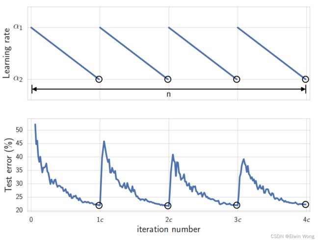
SWA is making use of multiple samples gathered through exploration of the set of points corresponding to high performing networks.** To enforce exploration we run SGD with constant or cyclical learning rates.**（为了加强与高性能网络相对应的权重集合的探索，以恒定或周期性的学习率执行SGD）

下面是两种学习率策略的计算公式：

• cyclical learning rate schedule: linearly decrease the learning rate from ${\alpha }_1$ to ${\alpha }_2$（在每个周期内线性地将学习率从${\alpha }_1$减少到${\alpha }_2$，一个周期为$c$个epoch）:

  $$\begin{array}{rl}\alpha (i)& =(1-t(i)){\alpha }_1+t(i){\alpha }_2,\\ t(i)& =\frac{1}{c}(\mathrm{mod}(i-1,c)+1)\end{array}$$

  

• constant learning rate schedule:

  $$\alpha (i)={\alpha }_1$$

When using a cyclical learning rate we capture the models $w_i$ that correspond to the minimum values of the learning rate. For constant learning rates we capture models at each epoch. Next, we average the weights of all the captured networks $w_i$ to get our final model $w_{SWA}$.

对于两种学习率调度策略，用于统计平均权重的模型是不同的。对于周期性的学习率而言，会使用对应于最小学习率的模型，也就是每个周期中最后一个epoch产生的模型；而对于恒定的学习率则比较简单，每个epoch的模型都会被用于计算平均权重。

The Algorithm

算法还是比较简单，就是对SGD产生的模型权重做等权重平均，这里就不做过多解释了，请看下面的算法步骤：

Batch normalization

If the DNN uses batch normalization, we run one additional pass over the data, as in Garipov et al. [2018], to compute the running mean and standard deviation of the activations for each layer of the network with $w_{SWA}$ weights after the training is finished, since these statistics are not collected during training. For most deep learning libraries, such as PyTorch or Tensorflow, one can typically collect these statistics by making a forward pass over the data in training mode.

最后需要注意的一点是，如果神经网络中用到了BN层，则需要在训练数据上再做一次额外的前向传播，用于计算BN层的均值、标准差这些统计信息，因为对于使用$w_{SWA}$权重的网络，在训练过程中是没有收集这些统计信息的。

在PyTorch中使用swa

最佳实践

上面是实践当中验证过的最佳的使用swa的方式，前面75%的训练时间使用标准的学习率衰减策略，后面的25%的训练实践使用比较高的恒定学习率，而最终的swa模型权重是由最后的25%训练时间中每个epoch得到的模型权重计算平均得到的。

Demo

下面是在PyTorch中使用swa的示例

from torch.optim.swa_utils import AveragedModel, SWALR
from torch.optim.lr_scheduler import CosineAnnealingLR

loader, optimizer, model, loss_fn = ...
swa_model = AveragedModel(model)
scheduler = CosineAnnealingLR(optimizer, T_max=100)
swa_start = 5
swa_scheduler = SWALR(optimizer, swa_lr=0.05)

for epoch in range(100):
      for input, target in loader:
          optimizer.zero_grad()
          loss_fn(model(input), target).backward()
          optimizer.step()
      if epoch > swa_start:
          swa_model.update_parameters(model)
          swa_scheduler.step()
      else:
          scheduler.step()

# Update bn statistics for the swa_model at the end
torch.optim.swa_utils.update_bn(loader, swa_model)
# Use swa_model to make predictions on test data 
preds = swa_model(test_input)