经典文献阅读之--Swin Transformer

0. 简介

Transfomer最近几年已经霸榜了各个领域，之前我们在《经典文献阅读之–Deformable DETR》这篇博客中对DETR这个系列进行了梳理，但是想着既然写了图像处理领域的方法介绍，正好也按照这个顺序来对另一个非常著名的Swin Transformer框架。Swin Transformer框架相较于传统Transformer精度和速度比CNN稍差，Swin Transformer可以说是CNN模型一个非常有力的替代方案。·下面是Swin Transformer在Github上的开源路径： https://github.com/microsoft/Swin-Transformer。

1. Swin Transformer创新性

我们在拿到这篇文章后，首先在开头就可以作者分析，当前的Transformer从NLP迁移到CV上没有大放异彩主要原因集中在：

1、 两个领域涉及的scale不同，NLP的scale是标准固定的，而CV的scale变化范围非常大。

2.、CV比起NLP需要更大的分辨率，而且CV中使用Transformer的计算复杂度是图像尺度的平方，这会导致计算量过于庞大。

而为了解决这两个问题，Swin Transformer相比之前的ViT做了两个改进：

1、引入CNN中常用的层次化构建方式构建层次化Transformer；

2、引入locality思想，对无重合的window区域内进行self-attention计算。

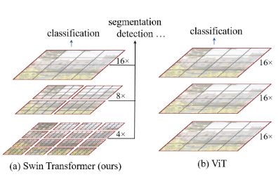
总的来说Swin Transformer是一种改进的VIT，但是Swin Transformer该模型本身具有了划窗操作（包括不重叠的local window，和重叠的cross-window），并且具有层级设计。

2. Swin Transformer的整体架构

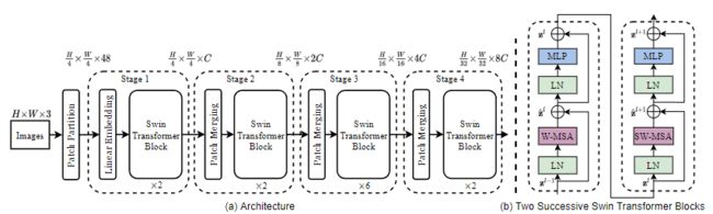
Swin Transformer的名字来自于Shifted window Transformer。这也凸显出了我们Swin Transformer在结构框架中的设计重点。整个Swin Transformer架构，和CNN架构非常相似，构建了4个stage，每个stage中都是类似的重复单元。下图为Swin Transformer总体设计架构。

2.1 Patch Partition

Swin Transformer第一步是Patch Partition模块。这一步和ViT相似，通过Patch Partition将输入图片$H\ast W\ast 3$划分为不重合的patch集合，其中每个patch尺寸为$4\ast 4$，那么每个patch的特征维度为$4\ast 4\ast 3=48$，patch块的数量为$H/4\ast W/4$。在代码中我们可以看到默认给定一张$224\ast 224\ast 3$的图片，经过patch partition后图片的尺寸为$56\ast 56\ast 48$（$56=224/4，48=16\ast 3$，3为RGB通道数）。

class SwinTransformer(nn.Module):
    r""" Swin Transformer
        A PyTorch impl of : `Swin Transformer: Hierarchical Vision Transformer using Shifted Windows`  -
          https://arxiv.org/pdf/2103.14030
    Args:
        img_size (int | tuple(int)): Input image size. Default 224
        patch_size (int | tuple(int)): Patch size. Default: 4
        in_chans (int): Number of input image channels. Default: 3
        num_classes (int): Number of classes for classification head. Default: 1000
        embed_dim (int): Patch embedding dimension. Default: 96
        depths (tuple(int)): Depth of each Swin Transformer layer.
        num_heads (tuple(int)): Number of attention heads in different layers.
        window_size (int): Window size. Default: 7
        mlp_ratio (float): Ratio of mlp hidden dim to embedding dim. Default: 4
        qkv_bias (bool): If True, add a learnable bias to query, key, value. Default: True
        qk_scale (float): Override default qk scale of head_dim ** -0.5 if set. Default: None
        drop_rate (float): Dropout rate. Default: 0
        attn_drop_rate (float): Attention dropout rate. Default: 0
        drop_path_rate (float): Stochastic depth rate. Default: 0.1
        norm_layer (nn.Module): Normalization layer. Default: nn.LayerNorm.
        ape (bool): If True, add absolute position embedding to the patch embedding. Default: False
        patch_norm (bool): If True, add normalization after patch embedding. Default: True
        use_checkpoint (bool): Whether to use checkpointing to save memory. Default: False
        fused_window_process (bool, optional): If True, use one kernel to fused window shift & window partition for acceleration, similar for the reversed part. Default: False
    """

    def __init__(self, img_size=224, patch_size=4, in_chans=3, num_classes=1000,
                 embed_dim=96, depths=[2, 2, 6, 2], num_heads=[3, 6, 12, 24],
                 window_size=7, mlp_ratio=4., qkv_bias=True, qk_scale=None,
                 drop_rate=0., attn_drop_rate=0., drop_path_rate=0.1,
                 norm_layer=nn.LayerNorm, ape=False, patch_norm=True,
                 use_checkpoint=False, fused_window_process=False, **kwargs):

2.2 Stage1—Linear Embedding

Stage1这部分的和后面三个Stage不一样，这里一开始是通过一个Linear Embedding将输入向量的维度变成预先设置好的值即Transformer能够接受的值C，然后送入Swin Transformer Block。这里在代码中我们可以看到超参数C设置为96。然后经过torch.flatten将图像拉直为$3136\ast 96$，$3136$就是序列的长度，$96$成为了每个token的维度。在Swin Transformer中的Patch Partition层和Linear Embedding层相当于ViT模型的Patch Projection层操作。

import torch
import torch.nn as nn


class PatchEmbed(nn.Module):
    def __init__(self, img_size=224, patch_size=4, in_chans=3, embed_dim=96, norm_layer=None):
        super().__init__()
        img_size = to_2tuple(img_size) # -> (img_size, img_size)
        patch_size = to_2tuple(patch_size) # -> (patch_size, patch_size)
        patches_resolution = [img_size[0] // patch_size[0], img_size[1] // patch_size[1]]
        self.img_size = img_size
        self.patch_size = patch_size
        self.patches_resolution = patches_resolution
        self.num_patches = patches_resolution[0] * patches_resolution[1]

        self.in_chans = in_chans
        self.embed_dim = embed_dim

        self.proj = nn.Conv2d(in_chans, embed_dim, kernel_size=patch_size, stride=patch_size)
        if norm_layer is not None:
            self.norm = norm_layer(embed_dim)
        else:
            self.norm = None

    def forward(self, x):
        # 假设采取默认参数
        x = self.proj(x) # 出来的是(N, 96, 224/4, 224/4) 
        x = torch.flatten(x, 2) # 把HW维展开，(N, 96, 56*56)
        x = torch.transpose(x, 1, 2)  # 把通道维放到最后 (N, 56*56, 96)
        if self.norm is not None:
            x = self.norm(x)
        return x

2.2 StageX—Patch Merging

该模块的作用是在每个Stage开始前做降采样，用于缩小分辨率，调整通道数 进而形成层次化的设计，同时也能节省一定运算量。下面是这部分的示意图：

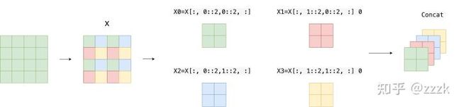
我们可以看到其实本质上就是对图像进行缩小并完成降采样的操作，即类似CNN中每个Stage开始前用stride=2的卷积/池化层的操作。在Swin-Transformer中就是通过间隔2来选取元素的操作，并concat到一起，作为一个张量，最后通道维度会变成原先的4倍。

最后再通过一个全连接层再调整通道维度为原来的两倍。对应的代码为：

class PatchMerging(nn.Module):
    def __init__(self, input_resolution, dim, norm_layer=nn.LayerNorm):
        super().__init__()
        self.input_resolution = input_resolution
        self.dim = dim
        self.reduction = nn.Linear(4 * dim, 2 * dim, bias=False)
        self.norm = norm_layer(4 * dim)

    def forward(self, x):
        """
        x: B, H*W, C
        """
        H, W = self.input_resolution
        B, L, C = x.shape
        assert L == H * W, "input feature has wrong size"
        assert H % 2 == 0 and W % 2 == 0, f"x size ({H}*{W}) are not even."

        x = x.view(B, H, W, C)

        x0 = x[:, 0::2, 0::2, :]  # B H/2 W/2 C
        x1 = x[:, 1::2, 0::2, :]  # B H/2 W/2 C
        x2 = x[:, 0::2, 1::2, :]  # B H/2 W/2 C
        x3 = x[:, 1::2, 1::2, :]  # B H/2 W/2 C
        x = torch.cat([x0, x1, x2, x3], -1)  # B H/2 W/2 4*C
        x = x.view(B, -1, 4 * C)  # B H/2*W/2 4*C

        x = self.norm(x)
        x = self.reduction(x)

        return x

2.3 Swin transformer块

Swin transformer中使用的块用Window MSA (W-MSA)和shift Window MSA (SW-MSA)模块取代了ViT中使用的标准多头自注意力(MSA)模块。Swin Transformer模块如下图所示

Swin transformer块有两个子单元。第一个单元使用W-MSA，第二个单元使用SW-MSA。每个子单元由一个规一化层、一个注意力模块、另一个规范化层和一个MLP层组成。第一个子单元使用Window Attention (W-MSA)模块，而第二个子单元使用Shifted Window Attention (SW-MSA)模块。

3. 算法具体细节

上面一章已经将最主要的三个模块讲完了，但是我们还没弄清楚这里面的关系，所以这一章详细的结合现有的方法，给读者梳理一下整个框架呈现出来的新Trick。

3.1 分层特征图

在经过四个Stage后最后我们可以看到，Swin Transformer中的分层特征映射。特征映射在每一层之后逐步合并和下采样，创建具有层次结构的特征映射。

同时由于分层特征映射的空间分辨率与ResNet中的相同。这样Swin Transformer就可以方便地在现有的视觉任务方法中替换ResNet骨干网络。

3.2 窗口级别的自注意力

ViT中使用的标准MSA执行全局自注意力，每个Patch之间的关系是根据所有其他Patch计算的。从而导致其不适合高分辨率的图像。

基于全局的自注意力计算会导致平方倍的复杂度，当进行视觉里的下游任务时尤其是密集预测型任务或者非常大尺寸的图片时，基于全局计算自注意力的复杂度会非常的高。比如我们在Stage拿到的序列长度就是3136，这相对于ViT模型里的196来说太长了，在这里就用到了基于窗口的自注意力，每个窗口都有7*7=49个小patch，所以序列长度就变成了49，这样就解决了计算复杂度的问题。

我们先简单看下公式，与传统Attention对比，主要区别是在原始计算Attention的公式中的Q,K时加入了相对位置编码。通过QK计算出来的Attention张量形状为(numWindows*B, num_heads, window_size*window_size, window_size*window_size)。
对于Attention张量来说，以不同元素为原点，其他元素的坐标也是不同的，以window_size=2为例，其相对位置编码如下图所示，如果想要深入了解Window Attention的，可以阅读这篇文章，已经讲得很详细了，这里就不照搬了。

下图为窗口大小为$2\ast 2$ patch，基于窗口的MSA只计算每个窗口内的注意力。

这展示了Swin Transformer算法中使用的窗口MSA只在每个窗口内计算注意力。

class WindowAttention(nn.Module):
    r""" Window based multi-head self attention (W-MSA) module with relative position bias.
    It supports both of shifted and non-shifted window.

    Args:
        dim (int): Number of input channels.
        window_size (tuple[int]): The height and width of the window.
        num_heads (int): Number of attention heads.
        qkv_bias (bool, optional):  If True, add a learnable bias to query, key, value. Default: True
        qk_scale (float | None, optional): Override default qk scale of head_dim ** -0.5 if set
        attn_drop (float, optional): Dropout ratio of attention weight. Default: 0.0
        proj_drop (float, optional): Dropout ratio of output. Default: 0.0
    """

    def __init__(self, dim, window_size, num_heads, qkv_bias=True, qk_scale=None, attn_drop=0., proj_drop=0.):

        super().__init__()
        self.dim = dim
        self.window_size = window_size  # Wh, Ww
        self.num_heads = num_heads # nH
        head_dim = dim // num_heads # 每个注意力头对应的通道数
        self.scale = qk_scale or head_dim ** -0.5

        # define a parameter table of relative position bias
        self.relative_position_bias_table = nn.Parameter(
            torch.zeros((2 * window_size[0] - 1) * (2 * window_size[1] - 1), num_heads))  # 设置一个形状为（2*(Wh-1) * 2*(Ww-1), nH）的可学习变量，用于后续的位置编码
  
        self.qkv = nn.Linear(dim, dim * 3, bias=qkv_bias)
        self.attn_drop = nn.Dropout(attn_drop)
        self.proj = nn.Linear(dim, dim)
        self.proj_drop = nn.Dropout(proj_drop)

        trunc_normal_(self.relative_position_bias_table, std=.02)
        self.softmax = nn.Softmax(dim=-1)
     # 相关位置编码...

…详情请参照古月居