【pytorch】nn.LSTM的使用

官方文档在这里。

LSTM具体不做介绍了，本篇只做pytorch的API使用介绍

torch.nn.LSTM(*args, **kwargs)

输入张量

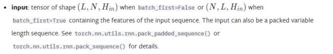
输入参数为两个，一个为input Tensor，一个为隐藏特征和状态组成的tuple

Inputs: input, (h_0, c_0)

input只能为3维张量，其中当初始参数batch_first=True时，shape为(L,N,H);而当初始参数batch_first=False时，shape为(N,L,H);

公式

LSTM中weights

以下公式介绍都忽略bias

• 公式(1), 输入门
  $i_t=\delta (W_{ii}{x}_t+W_{hi}{h}_{t-1})$， LSTM中有关输入的参是是$W_{ii}$和$W_{hi}$
• 公式(2),遗忘门
  $f_t=\delta (W_{if}{x}_t+W_{hf}{h}_{t-1})$, LSTM中有关输入的参数是$W_{if}$和$W_{hf}$
• 公式(3),细胞更新状态
  $g_t=\delta (W_{ig}{x}_t+W_{hg}{h}_{t-1})$, LSTM中有关输入的参数是$W_{ig}$和$W_{hg}$
• 公式(4),输出门
  $o_t=\delta (W_{io}{x}_t+W_{ho}{h}_{t-1})$, LSTM中有关输入的参数是$W_{io}$和$W_{ho}$

所以从输入张量和隐藏层张量来说，一共有两组参数

1. input 组 {$W_{ii}$， $W_{if}$，$W_{ig}$，$W_{io}$ }
2. hidden组 { $W_{hi}$，$W_{hf}$， $W_{hg}$， $W_{ho}$ }

这里就对应官网上的两个参数

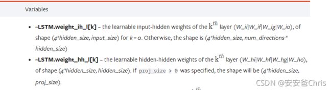
因为hidden size为隐藏层特征输出长度，所以每个参数第一维度都是hidden size；然后每一组是把4个张量按照第一维度拼接，所以要乘以4

举例代码：

from torch import nn

lstm = nn.LSTM(input_size=3, hidden_size=6, num_layers=1, bias=False)

print('weight_ih_l0.shape = ', lstm.weight_ih_l0.shape, ', weight_hh_l0.shape = ' , lstm.weight_hh_l0.shape)

双向LSTM

如果要实现双向的LSTM，只需要增加参数bidirectional=True

双向的区别是LTSM参数中 hidden 参数会增加一个方向，即有来有回，所以要double以下。

举例代码

from torch import nn

lstm = nn.LSTM(input_size=3, hidden_size=6, num_layers=2, bias=False, bidirectional=True)

print('weight_ih_l0.shape = ', lstm.weight_ih_l0.shape, ', weight_ih_l0_reverse.shape = ', lstm.weight_ih_l0_reverse.shape,
      '\nweight_hh_l0.shape = ' , lstm.weight_hh_l0.shape, ', weight_hh_l0_reverse.shape = ', lstm.weight_hh_l0_reverse.shape)

主要是hh部分的最后一维增加了一倍。

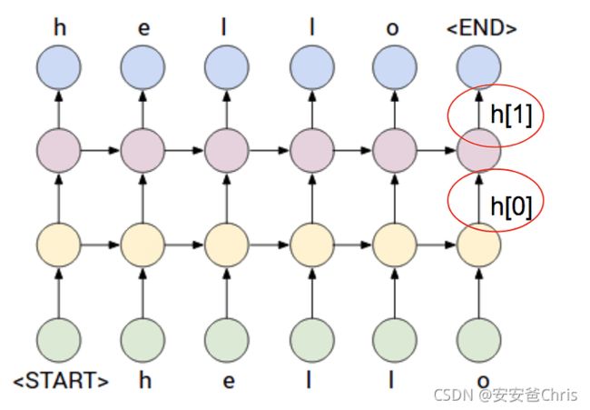
多层的概念

LSTM中有个参数num_layers是设置层数的，如果num_layers大于1,则网络则会变成如下的拓展

有关讨论请参考这里。

每多一层，就多一组**LSTM.weight_ih_l[k]和LSTM.weight_hh_l[k]**参数

两层的网络里有 LSTM.weight_ih_l0、LSTM.weight_ih_l0和LSTM.weight_ih_l1和LSTM.weight_hh_l1

---

LSTM的计算示例代码

input_size 为3，hidden_size 为4，

# shape [Sequence Length, Batch Size, Feature Size]
# 如果batch_first=True，则为 [Batch Size, Sequence Length, Feature Size]
x=torch.Tensor([0,0,1,1,1,1,0,0,0,0,0,0]).view(2,3,2)

print(x,x.shape)

# h0 c0 的三维度分别为 [Layer Size, Batch Size, Hidden Feature Size]
h0=torch.zeros(1,3,4)
c0=torch.zeros(1,3,4)

# 默认batch_first=False,所以输入张量的第1维度是Batch
net=nn.LSTM(2, 4, bias=False)
print("net.weight_ih_l0=", net.weight_ih_l0, net.weight_ih_l0.shape)
print("net.weight_hh_l0=", net.weight_hh_l0, net.weight_hh_l0.shape)
y,_=net(x, (h0,c0))
print(y, y.shape)

tensor([[[0., 0.],
         [1., 1.],
         [1., 1.]],

        [[0., 0.],
         [0., 0.],
         [0., 0.]]]) torch.Size([2, 3, 2])
net.weight_ih_l0= Parameter containing:
tensor([[-0.1310,  0.0330],
        [-0.3115, -0.0417],
        [-0.1452,  0.0426],
        [-0.0096,  0.3305],
        [-0.1104,  0.1816],
        [ 0.1668, -0.3706],
        [ 0.4792, -0.3867],
        [-0.4565,  0.0688],
        [ 0.0975, -0.0737],
        [ 0.2898,  0.2739],
        [-0.3564,  0.2723],
        [-0.1759,  0.2534],
        [ 0.3471, -0.1051],
        [ 0.4057,  0.3256],
        [ 0.4224,  0.4646],
        [-0.0107, -0.2000]], requires_grad=True) torch.Size([16, 2])
net.weight_hh_l0= Parameter containing:
tensor([[ 0.4431,  0.4195, -0.4328,  0.0183],
        [ 0.4375,  0.0306, -0.0641, -0.2027],
        [-0.3726, -0.0434, -0.4403,  0.2741],
        [-0.2962, -0.2381, -0.4713, -0.1349],
        [-0.1447, -0.0184,  0.3634, -0.0840],
        [-0.4828, -0.2628,  0.4112, -0.0554],
        [ 0.2004, -0.4253, -0.1785,  0.4688],
        [ 0.2922, -0.1926, -0.2644,  0.2561],
        [ 0.4504, -0.3577, -0.2971, -0.2796],
        [ 0.0442, -0.0018, -0.3970,  0.3194],
        [ 0.2986, -0.2493, -0.4371,  0.2953],
        [-0.0342, -0.2422, -0.2986,  0.0775],
        [ 0.4996,  0.1421, -0.1665,  0.1231],
        [-0.3341, -0.0462, -0.1578, -0.1443],
        [-0.0194,  0.3979,  0.0734, -0.2276],
        [ 0.0581, -0.3744,  0.4785, -0.0365]], requires_grad=True) torch.Size([16, 4])
tensor([[[ 0.0000,  0.0000,  0.0000,  0.0000],
         [ 0.0064,  0.1402, -0.0282,  0.0200],
         [ 0.0064,  0.1402, -0.0282,  0.0200]],

        [[ 0.0000,  0.0000,  0.0000,  0.0000],
         [-0.0089,  0.0553, -0.0138,  0.0050],
         [-0.0089,  0.0553, -0.0138,  0.0050]]], grad_fn=) torch.Size([2, 3, 4])

相关参考： Understanding LSTM and its diagram