CS231n笔记-CNN网络结构
所有图片来自PPT官网Index of /slides/2022
代码:Batch Normalization和Dropout_iwill323的博客-CSDN博客
目录
全连接层存在的问题
卷积层
卷积核学到了什么
超参数
1×1卷积层
pytorch
池化层
全连接层
Batch Normalization
为什么使用Batch Normalization
计算方式
全连接层的batch norm
卷积层的batch norm——spatial batchnorm
全连接层的Layer Normalization
Spatial Group Normalization
作用和问题
激活函数
Sigmoid
tanh(x)
Relu
Leaky ReLU
ELU
SELU
Maxout
使用建议
总结
全连接层存在的问题
在全连接层中,相邻层的神经元全部连接在一起,输出的数量可以任意决定。
全连接层存在什么问题呢?那就是数据的形状被“忽视”了。比如,输入数据是图像时,图像通常是高、长、通道方向上的 3 维形状。但是,向全连接层输入时,需要将 3 维数据拉平为 1 维数据。
图像是 3 维形状,这个形状中应该含有重要的空间信息。比如,空间上邻近的像素为相似的值、RBG 的各个通道之间分别有密切的关联性、相距较远的像素之间没有什么关联等,3 维形状中可能隐藏有值得提取的本质模式。但是,因为全连接层会忽视形状,将全部的输入数据作为相同的神经元(同一维度的神经元)处理,所以无法利用与形状相关的信息。
而卷积层可以保持形状不变。当输入数据是图像时,卷积层会以 3 维数据的形式接收输入数据,并同样以 3 维数据的形式输出至下一层。因此,在 CNN 中,可以(有可能)正确理解图像等具有形状的数据。
卷积层
卷积层使用卷积核与数据中与之相同大小(包括长、宽、深)的一组数据做内积,将其映射为一个数据(神经元neuron)。这块区域就是这个neuron的感受野receptive field。这与全连接层是显然不同的,在全连接层中,每个neuron和输入都是连接的。CNN 中,有时将卷积层的输入输出数据称为特征图(feature map)。其中,卷积层的输入数据称为输入特征图(input feature map),输出数据称为输出特征图(output feature map)
卷积神经网络中卷积核的高度和宽度通常为奇数,例如1、3、5或7。 选择奇数的好处是,保持空间维度的同时,我们可以在顶部和底部填充相同数量的行,在左侧和右侧填充相同数量的列。
此外,使用奇数的核大小和填充大小也提供了书写上的便利。对于任何二维张量X,当满足:
- 卷积核的大小是奇数;
- 所有边的填充行数和列数相同;
- 输出与输入具有相同高度和宽度
则可以得出:输出Y[i, j]是通过以输入X[i, j]为中心,与卷积核进行互相关计算得到的。
同一层的neuron共享一个卷积核,这样就大大减少了参数的数量。有时候共享参数是不合适的,具体参考官方笔记CS231n Convolutional Neural Networks for Visual Recognition

假设卷积核的尺寸保持为K×K,那么每经过一层卷积,一个neuron看到的感受野要加K-1,图片的信息就被不断压缩(提取)

可以使用多个卷积核,这样就能在一个卷积层上提取多个特征。注意每个卷积核的深度永远和数据深度相同;每个卷积核共享一个bias


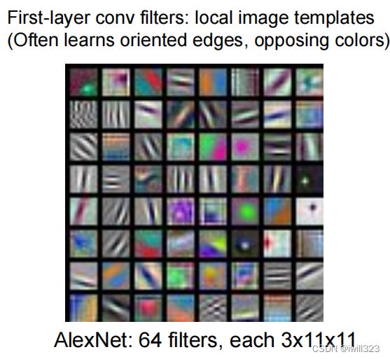
卷积核学到了什么
线性分类器对每一个分类学到了一个template,神经网络学到的template更为丰富
 |
 |
第一层卷积核学到的是最基本的特征,比如图像边缘。随着深度增加,每一层卷积层对上一层做综合,学习到更为复杂的特征(这一段是看图说话)
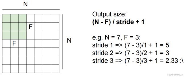
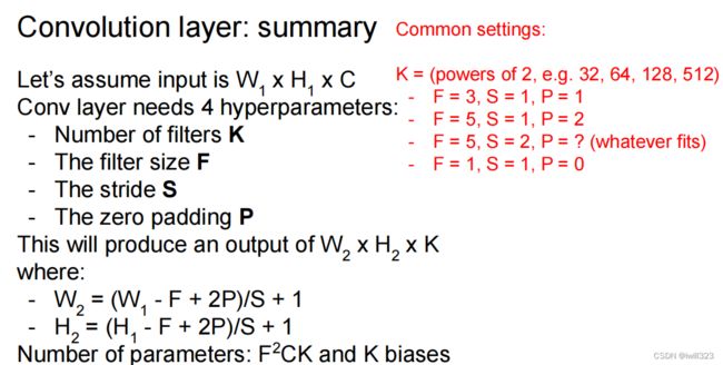
超参数
卷积核尺寸、滑动步长、padding、卷积核数量


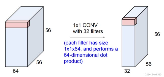
1×1卷积层
1×1卷积层是有用的,主要用于降低通道数量,进而降低参数数量
pytorch
pytorch的Conv2d函数,常数输入参数是这四个超参数(外加一个输入参数的通道)。输入输出如下:


池化层
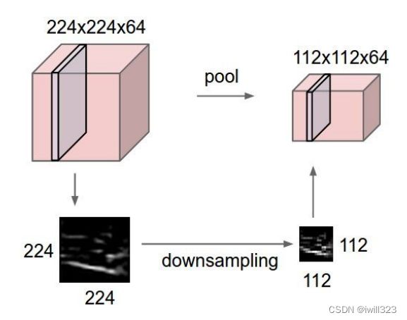
常用的是max pooling


全连接层
在卷积神经网络的最后往往跟一个全连接层,用于将学习到的特征映射到不同的分类
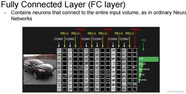
演示网站http://cs.stanford.edu/people/karpathy/convnetjs/demo/cifar10.html
Batch Normalization
为什么使用Batch Normalization
假设现在有一个非常简单的模型y=x1w1+x2w2+b,损失函数在两个参数上的梯度变化差别非常大,在w1方向上的斜率变化很小,在w2方向上面斜率变化很大,这样的模型难以进行训练(参考adaptive learning rate的部分)
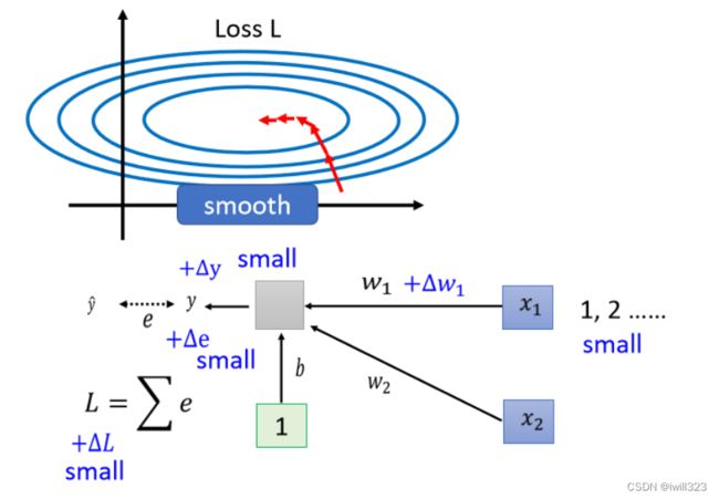
为什么w1和w2的斜率差别大?当自变量x2很大时,w2改变一点点,输出的y就会产生很大的差异,计算出来的 loss也会产生很大的差异,这就是w2方向上坡度陡峭的原因;而w1方向上坡度平缓的原因就是x1太小。综上可知:由于输入自变量 x 的量级不同,导致不同参数 w 的loss变化速度不同,也就形成了坡度不同的误差曲面。故而,为了使不同参数的loss 变化速度一样,只需要让自变量 x 全部处于同一量级上,这就叫做标准化

Batch Normalization的思路就是把难训练的误差曲面修改一下,改成容易进行训练的误差曲面。
当我们训练时,中间层中的变量也可能具有更⼴的变化范围。为此,要向神经网络中插入对数据分布进行正规化的层,即 Batch Normalization 层。通常插入在全连接层或者卷积层之后,非线性层之前。
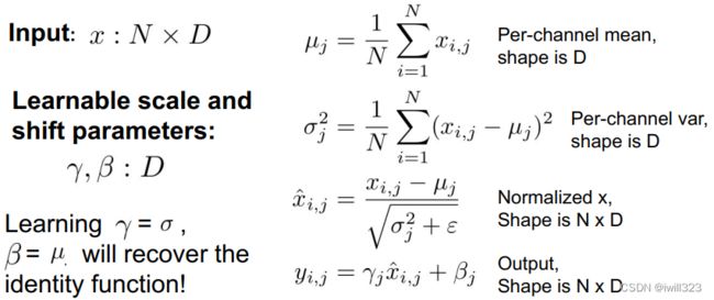
计算方式
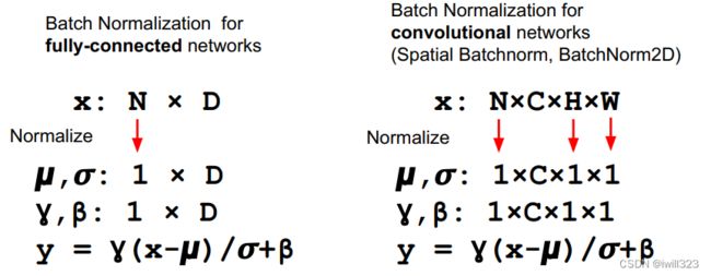
不同向量同一维度的元素放在一起计算。零均值、单位方差有可能会降低模型的表达能力,因此batch normalization层为特征值的每个维度引入缩放因子γ和平移因子β,通常刚开始设 γ=1,β=0,等到后面再改变γ,β的大小来调整 z 的分布,这两个参数让模型自己去学。
训练时,在实际操作的时候,不会让网络考虑整个训练集中的所有样本,一次只对一个batch 进行标准化。Batch Normalization有一个问题,它适用于 batch size 比较大的时候。如果batch size 中的数据足以表示整个数据集的分布,那就可以用这个batch的normalization代替整个数据集的normalization,作为近似值 。有一个够大的 batch,才算得出 μ和σ ,假设batch size 设为1,就没有计算μ和σ的必要了。
测试时没有batch,在训练过程中计算滑动平均,将滑动平均计算出来的μ和σ替换到原先的公式中(仍然要使用γ和β)
需要注意的是,μ和σ只能在训练集上评估,直接应用于验证集或测试集,而不是用整个数据集计算出μ和σ后,划分为训练集、验证集、测试集.
全连接层的batch norm
输入形状是(N, D) ,输出形状也是 (N, D),对每一列求均值 x_mean = np.mean(x, axis = 0)。通过移动平均估算整个训练数据集的样本均值和⽅差,并在预测时使⽤它们得到确定的输出
如果我们尝试使⽤⼤⼩为1的⼩批量应⽤批量规范化,我们将⽆法学到任何东西。这是因为在减去均值之后,每个隐藏单元将为0。所以,只有使⽤⾜够⼤的⼩批量,批量规范化这种⽅法才是有效且稳定的。在应⽤批量规范化时,批量⼤⼩的选择可能⽐没有批量规范化时更重要。
- 正向传播
def batchnorm_forward(x, gamma, beta, bn_param):
    """
    Input:
    - x: Data of shape (N, D)
    - gamma: Scale parameter of shape (D,)
    - beta: Shift paremeter of shape (D,)
    - bn_param: Dictionary with the following keys:
      - mode: 'train' or 'test'; required
      - eps: Constant for numeric stability
      - momentum: Constant for running mean / variance.
      - running_mean: Array of shape (D,) giving running mean of features
      - running_var Array of shape (D,) giving running variance of features

    Returns a tuple of:
    - out: of shape (N, D)
    - cache: A tuple of values needed in the backward pass
    """
    mode = bn_param["mode"]
    eps = bn_param.get("eps", 1e-5)
    momentum = bn_param.get("momentum", 0.9)

    N, D = x.shape
    running_mean = bn_param.get("running_mean", np.zeros(D, dtype=x.dtype))
    running_var = bn_param.get("running_var", np.zeros(D, dtype=x.dtype))

    out, cache = None, None
    if mode == "train":
        x_mean = np.mean(x, axis = 0)
        x_var = np.var(x, axis = 0) + eps
        x_norm = (x - x_mean) / np.sqrt(x_var)
        out = x_norm * gamma  + beta  #  (N, D)
        cache = (x, x_norm, gamma, x_mean, x_var)

        # Store the updated running means back into bn_param
        bn_param["running_mean"] = momentum * running_mean + (1 - momentum) * x_mean
        bn_param["running_var"] = momentum * running_var + (1 - momentum) * x_var

    elif mode == "test":
        x_norm = (x - running_mean) / np.sqrt(running_var + eps)
        out = gamma * x_norm + beta
    else:
        raise ValueError('Invalid forward batchnorm mode "%s"' % mode)

return out, cache- 反向传播
def batchnorm_backward_alt(dout, cache):
    x, x_norm, gamma, mean, var = cache
    std = np.sqrt(var)

    dgamma = np.sum(dout * x_norm, axis = 0)  #  (N, D) * (N, D)
    dbeta = np.sum(dout, axis = 0)

    N = 1.0 * x.shape[0]
    dfdu = dout * gamma
    # 将x_norm拆成x,mu,var三项,分别对x求导,然后加起来
    dfdv = np.sum(dfdu * (x - mean) * -0.5 * var ** -1.5, axis = 0) # f对var求导
    dfdw = np.sum(dfdu * -1 / std, axis = 0) + \
        dfdv * np.sum(-2/N * (x - mean), axis = 0)  # f对mu求导,包括var项对mu求导
    dx = dfdu / std + dfdv * 2/N * (x - mean) + dfdw / N  # 三项分别对x求导并求和

    return dx, dgamma, dbeta
卷积层的batch norm——spatial batchnorm
If the feature map was produced using convolutions, then we expect every feature channel's statistics e.g. mean, variance to be relatively consistent both between different images, and different locations within the same image -- after all, every feature channel is produced by the same convolutional filter! Therefore, spatial batch normalization computes a mean and variance for each of the C feature channels by computing statistics over the minibatch dimension N as well the spatial dimensions H and W. 当卷积有多个输出通道时,我们需要对这些通道的“每个”输出执⾏批量规范化,假设我们的⼩批量包含m个样本,并且对于每个通道,卷积的输出具有⾼度p和宽度q。那么对于卷积层,我们在每个输出通道的m · p · q个元素上同时执⾏每个批量规范化
Sergey Ioffe and Christian Szegedy, "Batch Normalization: Accelerating Deep Network Training by Reducing Internal Covariate Shift", ICML 2015.
- 正向传播
def spatial_batchnorm_forward(x, gamma, beta, bn_param):
    """
    Inputs:
    - x: Input data of shape (N, C, H, W)
    - gamma: Scale parameter, of shape (C,)
    - beta: Shift parameter, of shape (C,)
    - bn_param: Dictionary with the following keys:
      - mode: 'train' or 'test'; required
      - eps: Constant for numeric stability
      - momentum: Constant for running mean / variance. momentum=0 means that
        old information is discarded completely at every time step, while
        momentum=1 means that new information is never incorporated. The
        default of momentum=0.9 should work well in most situations.
      - running_mean: Array of shape (D,) giving running mean of features
      - running_var Array of shape (D,) giving running variance of features

    Returns a tuple of:
    - out: Output data, of shape (N, C, H, W)
    - cache: Values needed for the backward pass
    """
    out, cache = None, None
    N, C, H, W = x.shape
    x_trans = x.transpose(0,2,3,1).reshape(N*H*W, C)  # 对每一个C进行归一化
    out1, cache = batchnorm_forward(x_trans, gamma, beta, bn_param)
    out = out1.reshape(N, H, W, C).transpose(0,3,1,2)

return out, cache- 反向传播
def spatial_batchnorm_backward(dout, cache):
    """Computes the backward pass for spatial batch normalization.

    Inputs:
    - dout: Upstream derivatives, of shape (N, C, H, W)
    - cache: Values from the forward pass

    Returns a tuple of:
    - dx: Gradient with respect to inputs, of shape (N, C, H, W)
    - dgamma: Gradient with respect to scale parameter, of shape (C,)
    - dbeta: Gradient with respect to shift parameter, of shape (C,)
    """
    N, C, H, W = dout.shape
    dout_trans = dout.transpose(0,2,3,1).reshape(N*H*W, C)
    dx, dgamma, dbeta = batchnorm_backward_alt(dout_trans, cache)
    dx = dx.reshape(N, H, W, C).transpose(0,3,1,2)

    return dx, dgamma, dbeta
全连接层的Layer Normalization
鉴于batch norm中batch size的影响较大,可以在每一个样本内求均值,避免N的影响。各个样本内求均值 x_mean = np.mean(x, axis = 1, keepdims = True)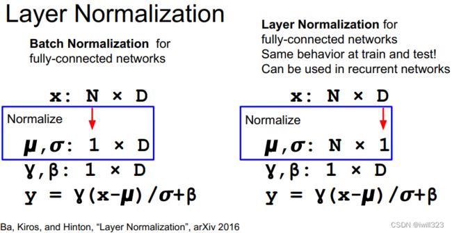
def layernorm_forward(x, gamma, beta, ln_param):
    """
    Note that in contrast to batch normalization, the behavior during train and test-time for
    layer normalization are identical, and we do not need to keep track of running averages
    of any sort.

    Input:
    - x: Data of shape (N, D)
    - gamma: Scale parameter of shape (D,)
    - beta: Shift paremeter of shape (D,)
    - ln_param: Dictionary with the following keys:
        - eps: Constant for numeric stability

    Returns a tuple of:
    - out: of shape (N, D)
    - cache: A tuple of values needed in the backward pass
    """
    out, cache = None, None
    eps = ln_param.get("eps", 1e-5)

    x_mean = np.mean(x, axis = 1, keepdims = True)
    x_var = np.var(x, axis = 1, keepdims = True) + eps
    x_std = np.sqrt(x_var)
    x_norm = (x - x_mean) / x_std
    out = x_norm *gamma + beta
    cache = (gamma, x, x_norm, x_mean, x_var)
    return out, cache

def layernorm_backward(dout, cache):
    gamma,x, x_norm,  mean, var = cache
    std = np.sqrt(var)
    dgamma = np.sum(dout * x_norm, axis = 0)
    dbeta = np.sum(dout, axis = 0)

    D = 1.0 * x.shape[1]
    dfdu = dout * gamma
    dfdv = np.sum(dfdu * (x - mean) * -0.5 * var ** -1.5, axis = 1)
    dfdw = np.sum(dfdu * -1 / std, axis = 1) + dfdv * np.sum(-2/D * (x - mean), axis = 1)
    # dfdv 和 dfdw.shape的形状都是(N,) dfdv.reshape(-1, 1)形状是(N,1)
    dx = dfdu / std + dfdv.reshape(-1, 1) * 2/D * (x - mean) + dfdw.reshape(-1, 1) / D
    return dx, dgamma, dbeta
Spatial Group Normalization
as the authors of [1] observed, Layer Normalization does not perform as well as Batch Normalization when used with Convolutional Layers:
With fully connected layers, all the hidden units in a layer tend to make similar contributions to the final prediction, and re-centering and rescaling the summed inputs to a layer works well. However, the assumption of similar contributions is no longer true for convolutional neural networks. The large number of the hidden units whose receptive fields lie near the boundary of the image are rarely turned on and thus have very different statistics from the rest of the hidden units within the same layer.
The authors of [2] propose an intermediary technique. In contrast to Layer Normalization, where you normalize over the entire feature per-datapoint, they suggest a consistent splitting of each per-datapoint feature into G groups and a per-group per-datapoint normalization instead.
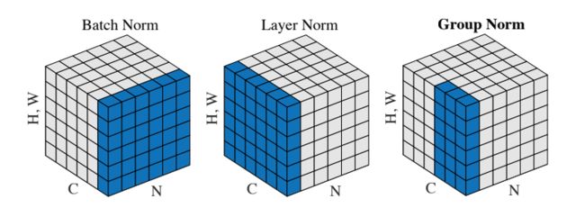
Even though an assumption of equal contribution is still being made within each group, the authors hypothesize that this is not as problematic, as innate grouping arises within features for visual recognition. One example they use to illustrate this is that many high-performance handcrafted features in traditional computer vision have terms that are explicitly grouped together. Take for example Histogram of Oriented Gradients [3] -- after computing histograms per spatially local block, each per-block histogram is normalized before being concatenated together to form the final feature vector.
Ba, Jimmy Lei, Jamie Ryan Kiros, and Geoffrey E. Hinton. "Layer Normalization." stat 1050 (2016): 21.
Wu, Yuxin, and Kaiming He. "Group Normalization." arXiv preprint arXiv:1803.08494 (2018).
N. Dalal and B. Triggs. Histograms of oriented gradients for human detection. In Computer Vision and Pattern Recognition (CVPR), 2005.
- 正向传播
def spatial_groupnorm_forward(x, gamma, beta, G, gn_param):
    """
    Inputs:
    - x: Input data of shape (N, C, H, W)
    - gamma: Scale parameter, of shape (1, C, 1, 1)
    - beta: Shift parameter, of shape (1, C, 1, 1)
    - G: Integer mumber of groups to split into, should be a divisor of C
    - gn_param: Dictionary with the following keys:
      - eps: Constant for numeric stability

    Returns a tuple of:
    - out: Output data, of shape (N, C, H, W)
    - cache: Values needed for the backward pass
    """
    out, cache = None, None
    eps = gn_param.get("eps", 1e-5)

    N, C, H, W = x.shape
    x_trans = x.reshape(N, G, C//G, H, W)
    mean = np.mean(x_trans, axis = (2,3,4), keepdims = True)
    var = np.var(x_trans, axis = (2,3,4), keepdims = True) + eps
    std = np.sqrt(var)
    x_norm = (x_trans - mean) / std
    x_norm = x_norm.reshape(x.shape)
    out = x_norm * gamma + beta

    cache = (x, x_norm, gamma, mean, var, std, G)

return out, cache- 反向传播
def spatial_groupnorm_backward(dout, cache):
    """
    Inputs:
    - dout: Upstream derivatives, of shape (N, C, H, W)
    - cache: Values from the forward pass

    Returns a tuple of:
    - dx: Gradient with respect to inputs, of shape (N, C, H, W)
    - dgamma: Gradient with respect to scale parameter, of shape (1, C, 1, 1)
    - dbeta: Gradient with respect to shift parameter, of shape (1, C, 1, 1)
    """
    dx, dgamma, dbeta = None, None, None

    x, x_norm, gamma, mean, var, std, G = cache
    N, C, H, W = x.shape
    dgamma = np.sum(dout * x_norm, axis = (0,2,3))[None, :, None, None]
    dbeta = np.sum(dout, axis = (0,2,3))[None, :, None, None]
    x_trans = x.reshape(N, G, C//G, H, W)

    M = C // G * H * W
    dfdu = (dout * gamma).reshape(N, G, C//G, H, W)
    dfdv = np.sum(dfdu * (x_trans - mean) * -0.5 * var ** -1.5, axis = (2,3,4))
    dfdw = np.sum(dfdu * -1 / std, axis = (2,3,4)) + dfdv * np.sum(-2/N * (x_trans - mean), axis = (2,3,4))
    dx = dfdu / std + dfdv.reshape(N, G, 1, 1, 1) * 2/M * (x_trans - mean) + dfdw.reshape(N, G, 1, 1, 1) / M
    dx = dx.reshape(x.shape)
    return dx, dgamma, dbeta
作用和问题
- 能够使用更大的学习率,收敛更快。
- 网络对初始化的鲁棒性更强
图中的实线是使用了 Batch Norm 时的结果,虚线是没有使用 Batch Norm 时的结果。图的标题处标明了权重初始值的标准差。几乎所有的情况下都是使用 Batch Norm 时学习进行得更快,在不使用 Batch Norm 的情况下,如果不赋予一个尺度好的初始值,学习将完全无法进行。
可见,通过使用 Batch Norm,可以推动学习的进行。并且,对权重初始值变得健壮(不那么依赖初始值)。

- 在训练过程中起到正则化的作用
每个样本通过batch均值和方差受同一batch其他样本的影响,引入了噪音,有正则化的作用(降低 Dropout 等的必要性)
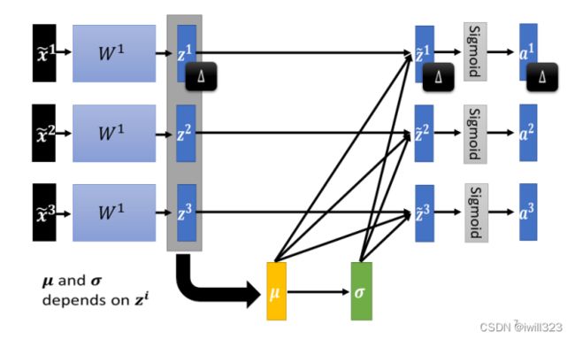
μ和σ都是由z1、z2、z3得到的,进行normalization之后,z1、z2、z3的值就发生改变了,从而改变了a1、a2、a3的值。在原先的处理过程中,x1、x2、x3是独立分开处理的,但是我们在做normalization 以后,这三个example变得彼此有关联了。
- Zero overhead at test-time: can be fused with conv!
- Behaves differently during training and testing: this is a very common source of bugs!
代码参见:Batch Normalization和Dropout_iwill323的博客-CSDN博客
激活函数
Sigmoid
存在的问题有:
1.梯度消失。当x的绝对值比较大的时候(如下图),梯度几乎为0,导致权重不再更新了。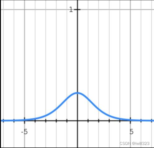
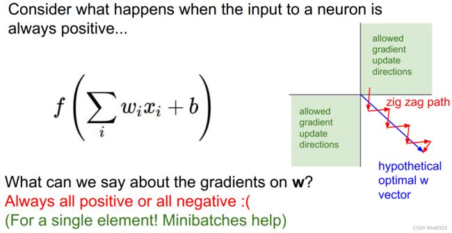
2.激活结果不是以0为均值。neuron的输入都是正的,于是局部梯度也是正的,所有的梯度都是一个符号。打个比方,有的卷积层权重应该增加,有的卷积层权重应该减少,但是现在所有权重在一次更新中都增加或都减小,本来一步到位的更新(下面第二张图的蓝线),需要很多步才能达到(zig-zagging dynamics in the gradient update),显然更新过程走了弯路。不过在一次batch计算中,每一层的梯度是要做求和运算的,这样梯度符号也会起变化,所以这个问题还好一点。

3.exp() 计算相对有些复杂
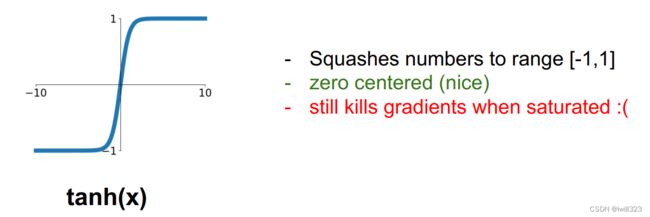
tanh(x)
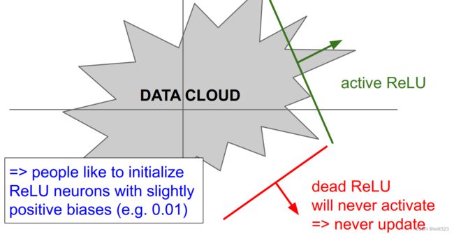
Relu
最大的问题在于负x区间内,权重梯度为0,意味着它反向传播中不再更新了,这个neuron“死掉”了。如果学习率太大或者初始化不好,会出现这样的问题

Leaky ReLU
由于x负区间有数值,所以neuron不会死。负区间的斜率可以当做一个参数来学习,参考Delving Deep into Rectifiers PReLU neurons
ELU

SELU

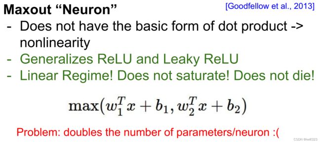
Maxout
使用建议
- Use ReLU. Be careful with your learning rates
- Try out Leaky ReLU / Maxout / ELU / SELU
- To squeeze out some marginal gains
- Don’t use sigmoid or tanh
总结

PPT最后给出的总结,与其说是总结,不如说挖了很多的坑,比如为什么要使用更小的卷积核,为什么趋向于不是用池化层/FC层,官方笔记有讲解CS231n Convolutional Neural Networks for Visual Recognition
也可以参考下面网页,写的挺不错的神经网络:全连接层转换为卷积层_AntheLinZ的博客-CSDN博客_全连接层转化为卷积层
全连接层转化为卷积层_写个翻译的博客-CSDN博客_全连接层转化为卷积层