基于pytorch的胶囊网络minst图像分类实现

关于《Dynamic Routing Between Capsules》这篇论文的代码复现网上有很多，基本都是做图像重构的。我修改了其中一部分代码，实现了minst图像分类。
参考：基于pytorch的CapsNet代码详解.

胶囊网络结构

胶囊网络基本结构如下：

• 普通卷积层conv1
• 预胶囊层PrimaryCaps：为胶囊层做准备，运算为卷积运算。
• 胶囊层DigitCaps：代替全连接层，输出为10个胶囊。

图像重构和图像分类不同的是，胶囊层后面还接了一个decoder层，将输出的胶囊转化为图像，所以前面的代码都是一样的。下面我们直接来看分类的实现。

package

import torch
from torch import nn
from torch.optim import Adam
import torch.nn.functional as F
from torchvision import transforms, datasets
import time

dataset

def load_mnist(path='./data', download=False, batch_size=100, shift_pixels=2):
    """
    Construct dataloaders for training and test data. Data augmentation is also done here.
    :param path: file path of the dataset
    :param download: whether to download the original data
    :param batch_size: batch size
    :param shift_pixels: maximum number of pixels to shift in each direction
    :return: train_loader, test_loader
    """
    kwargs = {'num_workers': 1, 'pin_memory': True}

    train_loader = torch.utils.data.DataLoader(
        datasets.MNIST(path, train=True, download=download,
                       transform=transforms.ToTensor()),
        batch_size=batch_size, shuffle=True, **kwargs)

    test_loader = torch.utils.data.DataLoader(
        datasets.MNIST(path, train=False, download=download,
                       transform=transforms.ToTensor()),
        batch_size=batch_size, shuffle=True, **kwargs)

    return train_loader, test_loader

model

1）Sqush激活函数

def squash(inputs, axis=-1):
    """
    The non-linear activation used in Capsule. It drives the length of a large vector to near 1 and small vector to 0
    :param inputs: vectors to be squashed
    :param axis: the axis to squash
    :return: a Tensor with same size as inputs
    """
    norm = torch.norm(inputs, p=2, dim=axis, keepdim=True)
    scale = norm**2 / (1 + norm**2) / (norm + 1e-8)
    return scale * inputs

此函数用来将verctor（胶囊就是vector）的长度（范数）压缩到0和1之间，axis=-1表示压缩倒数第一维。

2） PrimaryCapsule

class PrimaryCapsule(nn.Module):
    """
    Apply Conv2D with `out_channels` and then reshape to get capsules
    :param in_channels: input channels
    :param out_channels: output channels
    :param dim_caps: dimension of capsule
    :param kernel_size: kernel size
    :return: output tensor, size=[batch, num_caps, dim_caps]
    """
    def __init__(self, in_channels, out_channels, dim_caps, kernel_size, stride=1, padding=0):
        super(PrimaryCapsule, self).__init__()
        self.dim_caps = dim_caps
        self.conv2d = nn.Conv2d(in_channels, out_channels, kernel_size=kernel_size, stride=stride, padding=padding)

    def forward(self, x):
        outputs = self.conv2d(x)
        outputs = outputs.view(x.size(0), -1, self.dim_caps)
        return squash(outputs)

预胶囊层：

• num_caps是胶囊个数，dim_caps是胶囊维度。
• output size为[batch, num_caps, dim_caps]。

3） DenseCapsule

class DenseCapsule(nn.Module):
    """
    The dense capsule layer. It is similar to Dense (FC) layer. Dense layer has `in_num` inputs, each is a scalar, the
    output of the neuron from the former layer, and it has `out_num` output neurons. DenseCapsule just expands the
    output of the neuron from scalar to vector. So its input size = [None, in_num_caps, in_dim_caps] and output size = \
    [None, out_num_caps, out_dim_caps]. For Dense Layer, in_dim_caps = out_dim_caps = 1.

    :param in_num_caps: number of cpasules inputted to this layer
    :param in_dim_caps: dimension of input capsules
    :param out_num_caps: number of capsules outputted from this layer
    :param out_dim_caps: dimension of output capsules
    :param routings: number of iterations for the routing algorithm
    """
    def __init__(self, in_num_caps, in_dim_caps, out_num_caps, out_dim_caps, routings=3):
        super(DenseCapsule, self).__init__()
        self.in_num_caps = in_num_caps
        self.in_dim_caps = in_dim_caps
        self.out_num_caps = out_num_caps
        self.out_dim_caps = out_dim_caps
        self.routings = routings
        self.weight = nn.Parameter(0.01 * torch.randn(out_num_caps, in_num_caps, out_dim_caps, in_dim_caps))

    def forward(self, x):
        x_hat = torch.squeeze(torch.matmul(self.weight, x[:, None, :, :, None]), dim=-1)
        x_hat_detached = x_hat.detach()

        # The prior for coupling coefficient, initialized as zeros.
        # b.size = [batch, out_num_caps, in_num_caps]
        b = torch.zeros(x.size(0), self.out_num_caps, self.in_num_caps)

        assert self.routings > 0, 'The \'routings\' should be > 0.'
        for i in range(self.routings):
            # c.size = [batch, out_num_caps, in_num_caps]
            c = F.softmax(b, dim=1)

            # At last iteration, use `x_hat` to compute `outputs` in order to backpropagate gradient
            if i == self.routings - 1:
                # c.size expanded to [batch, out_num_caps, in_num_caps, 1           ]
                # x_hat.size     =   [batch, out_num_caps, in_num_caps, out_dim_caps]
                # => outputs.size=   [batch, out_num_caps, 1,           out_dim_caps]
                outputs = squash(torch.sum(c[:, :, :, None] * x_hat, dim=-2, keepdim=True))
                # outputs = squash(torch.matmul(c[:, :, None, :], x_hat))  # alternative way
            else:  # Otherwise, use `x_hat_detached` to update `b`. No gradients flow on this path.
                outputs = squash(torch.sum(c[:, :, :, None] * x_hat_detached, dim=-2, keepdim=True))
                # outputs = squash(torch.matmul(c[:, :, None, :], x_hat_detached))  # alternative way

                # outputs.size       =[batch, out_num_caps, 1,           out_dim_caps]
                # x_hat_detached.size=[batch, out_num_caps, in_num_caps, out_dim_caps]
                # => b.size          =[batch, out_num_caps, in_num_caps]
                b = b + torch.sum(outputs * x_hat_detached, dim=-1)

        return torch.squeeze(outputs, dim=-2)

这一步即胶囊层DigitCaps。

• input size：[batch, in_num_caps, in_dim_caps]，经x[: , None , : , : , None]扩展后维度为[batch, 1, in_num_caps, in_dim_caps, 1]。
• torch.matmul将扩展后的输入和weight 相乘后得 [batch, out_num_caps, in_num_caps,out_dim_caps, 1]，压缩后得 [batch,out_num_caps,in_num_caps,out_dim_caps]。
  torch.matmul()用法介绍.
• 动态路由算法部分：
  
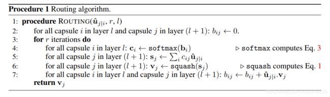
• 前几次迭代用的是x_hat_detached（切断反向传播），最后一次用的是x_hat，原因只有最后一次迭代得到的胶囊才会用作下一层的输入，需要加到计算图里。
• outputs size为[batch, out_num_caps, in_num_caps]。胶囊之间相连接。

4）CapsuleNet

class CapsuleNet(nn.Module):
    """
    A Capsule Network on MNIST.
    :param input_size: data size = [channels, width, height]
    :param classes: number of classes
    :param routings: number of routing iterations
    Shape:
        - Input: (batch, channels, width, height), optional (batch, classes) .
        - Output:((batch, classes), (batch, channels, width, height))
    """

    def __init__(self, input_size, classes, routings):
        super(CapsuleNet, self).__init__()
        self.input_size = input_size
        self.classes = classes
        self.routings = routings

        # Layer 1: Just a conventional Conv2D layer
        self.conv1 = nn.Conv2d(
            input_size[0], 256, kernel_size=9, stride=1, padding=0)

        # Layer 2: Conv2D layer with `squash` activation, then reshape to [None, num_caps, dim_caps]
        self.primarycaps = PrimaryCapsule(
            256, 256, 8, kernel_size=9, stride=2, padding=0)

        # Layer 3: Capsule layer. Routing algorithm works here.
        self.digitcaps = DenseCapsule(in_num_caps=32*6*6, in_dim_caps=8,
                                      out_num_caps=classes, out_dim_caps=16, routings=routings)

        self.relu = nn.ReLU()

    def forward(self, x, y=None):
        x = self.relu(self.conv1(x))
        x = self.primarycaps(x)
        x = self.digitcaps(x)
        length = x.norm(dim=-1)
        return length

Capsulenet类是前面各个module的组合。最终的输出是10个胶囊的范数。

train

计算准确率的函数：

def evaluate_accuracy(data_iter, net):
    acc_sum, n = 0.0, 0
    with torch.no_grad():
        for X, y in data_iter:
            if isinstance(net, torch.nn.Module):
                net.eval() # 评估模式, 这会关闭dropout
                acc_sum += (net(X).argmax(dim=1) == y).float().sum().item()
                net.train() # 改回训练模式
            else: 
                if('is_training' in net.__code__.co_varnames): # 如果有is_training这个参数
                    # 将is_training设置成False
                    acc_sum += (net(X, is_training=False).argmax(dim=1) == y).float().sum().item() 
                else:
                    acc_sum += (net(X).argmax(dim=1) == y).float().sum().item() 
            n += y.shape[0]
    return acc_sum / n

训练过程：

def train(train_iter, test_iter, net, loss, optimizer, num_epochs):
    batch_count = 0
    for epoch in range(num_epochs):
        train_l_sum, train_acc_sum, n, start = 0.0, 0.0, 0, time.time()
        for X, y in train_iter:
            y_hat = net(X)
            l = loss(y_hat, y)
            optimizer.zero_grad()
            l.backward()
            optimizer.step()
            train_l_sum += l.item()
            train_acc_sum += (y_hat.argmax(dim=1) == y).sum().item()
            n += y.shape[0]
            batch_count += 1
        test_acc = evaluate_accuracy(test_iter, net)
        print(
            'epoch %d, loss %.4f, train acc %.3f, test acc %.3f, time %.1f sec'
            % (epoch + 1, train_l_sum / batch_count, train_acc_sum / n,
               test_acc, time.time() - start))

batch_size, lr, num_epochs = 100, 0.001, 5
# load dat
train_iter, test_iter = load_mnist('./data', download=False, batch_size=batch_size)
# define model
net = CapsuleNet(input_size=[1, 28, 28], classes=10, routings=3)

optimizer = torch.optim.Adam(net.parameters(), lr=lr)
loss = nn.CrossEntropyLoss()
train(train_iter, test_iter, net, loss, optimizer, num_epochs)

result

训练时长再破记录，一个epoch就跑了两个多小时，我已经没有耐心等它跑完了。不过胶囊网络的确有这个特点，参数少，但训练慢。
效果其实很明显了，两个epoch准确率就达到了98.3%。
论文里给出的数据如下：

错误率0.25%，比CNN表现好。

ps：关于代码细节可以去看我参考的那篇博客和源代码，里面讲的挺详细的。