- 机器学习与深度学习间关系与区别
ℒℴѵℯ心·动ꦿ໊ོ꫞
人工智能学习深度学习python
一、机器学习概述定义机器学习(MachineLearning,ML)是一种通过数据驱动的方法,利用统计学和计算算法来训练模型,使计算机能够从数据中学习并自动进行预测或决策。机器学习通过分析大量数据样本,识别其中的模式和规律,从而对新的数据进行判断。其核心在于通过训练过程,让模型不断优化和提升其预测准确性。主要类型1.监督学习(SupervisedLearning)监督学习是指在训练数据集中包含输入
- 探索OpenAI和LangChain的适配器集成:轻松切换模型提供商
nseejrukjhad
langchaineasyui前端python
#探索OpenAI和LangChain的适配器集成:轻松切换模型提供商##引言在人工智能和自然语言处理的世界中,OpenAI的模型提供了强大的能力。然而,随着技术的发展,许多人开始探索其他模型以满足特定需求。LangChain作为一个强大的工具,集成了多种模型提供商,通过提供适配器,简化了不同模型之间的转换。本篇文章将介绍如何使用LangChain的适配器与OpenAI集成,以便轻松切换模型提供商
- 深入理解 MultiQueryRetriever:提升向量数据库检索效果的强大工具
nseejrukjhad
数据库python
深入理解MultiQueryRetriever:提升向量数据库检索效果的强大工具引言在人工智能和自然语言处理领域,高效准确的信息检索一直是一个关键挑战。传统的基于距离的向量数据库检索方法虽然广泛应用,但仍存在一些局限性。本文将介绍一种创新的解决方案:MultiQueryRetriever,它通过自动生成多个查询视角来增强检索效果,提高结果的相关性和多样性。MultiQueryRetriever的工
- 人工智能时代,程序员如何保持核心竞争力?
jmoych
人工智能
随着AIGC(如chatgpt、midjourney、claude等)大语言模型接二连三的涌现,AI辅助编程工具日益普及,程序员的工作方式正在发生深刻变革。有人担心AI可能取代部分编程工作,也有人认为AI是提高效率的得力助手。面对这一趋势,程序员应该如何应对?是专注于某个领域深耕细作,还是广泛学习以适应快速变化的技术环境?又或者,我们是否应该将重点转向AI无法轻易替代的软技能?让我们一起探讨程序员
- 数字里的世界17期:2021年全球10大顶级数据中心,中国移动榜首
张三叨
你知道吗?2016年,全球的数据中心共计用电4160亿千瓦时,比整个英国的发电量还多40%!前言每天,我们都会创造超过250万TB的数据。并且随着物联网(IOT)的不断普及,这一数据将持续增长。如此庞大的数据被存储在被称为“数据中心”的专用设施中。虽然最早的数据中心建于20世纪40年代,但直到1997-2000年的互联网泡沫期间才逐渐成为主流。当前人类的技术,比如人工智能和机器学习,已经将我们推向
- nosql数据库技术与应用知识点
皆过客,揽星河
NoSQLnosql数据库大数据数据分析数据结构非关系型数据库
Nosql知识回顾大数据处理流程数据采集(flume、爬虫、传感器)数据存储(本门课程NoSQL所处的阶段)Hdfs、MongoDB、HBase等数据清洗(入仓)Hive等数据处理、分析(Spark、Flink等)数据可视化数据挖掘、机器学习应用(Python、SparkMLlib等)大数据时代存储的挑战(三高)高并发(同一时间很多人访问)高扩展(要求随时根据需求扩展存储)高效率(要求读写速度快)
- Python开发常用的三方模块如下:
换个网名有点难
python开发语言
Python是一门功能强大的编程语言,拥有丰富的第三方库,这些库为开发者提供了极大的便利。以下是100个常用的Python库,涵盖了多个领域:1、NumPy,用于科学计算的基础库。2、Pandas,提供数据结构和数据分析工具。3、Matplotlib,一个绘图库。4、Scikit-learn,机器学习库。5、SciPy,用于数学、科学和工程的库。6、TensorFlow,由Google开发的开源机
- 简单了解 JVM
记得开心一点啊
jvm
目录♫什么是JVM♫JVM的运行流程♫JVM运行时数据区♪虚拟机栈♪本地方法栈♪堆♪程序计数器♪方法区/元数据区♫类加载的过程♫双亲委派模型♫垃圾回收机制♫什么是JVMJVM是JavaVirtualMachine的简称,意为Java虚拟机。虚拟机是指通过软件模拟的具有完整硬件功能的、运行在一个完全隔离的环境中的完整计算机系统(如:JVM、VMwave、VirtualBox)。JVM和其他两个虚拟机
- Python实现简单的机器学习算法
master_chenchengg
pythonpython办公效率python开发IT
Python实现简单的机器学习算法开篇:初探机器学习的奇妙之旅搭建环境:一切从安装开始必备工具箱第一步:安装Anaconda和JupyterNotebook小贴士:如何配置Python环境变量算法初体验:从零开始的Python机器学习线性回归:让数据说话数据准备:从哪里找数据编码实战:Python实现线性回归模型评估:如何判断模型好坏逻辑回归:从分类开始理论入门:什么是逻辑回归代码实现:使用skl
- JVM、JRE和 JDK:理解Java开发的三大核心组件
Y雨何时停T
Javajava
Java是一门跨平台的编程语言,它的成功离不开背后强大的运行环境与开发工具的支持。在Java的生态中,JVM(Java虚拟机)、JRE(Java运行时环境)和JDK(Java开发工具包)是三个至关重要的核心组件。本文将探讨JVM、JDK和JRE的区别,帮助你更好地理解Java的运行机制。1.JVM:Java虚拟机(JavaVirtualMachine)什么是JVM?JVM,即Java虚拟机,是Ja
- 遥感影像的切片处理
sand&wich
计算机视觉python图像处理
在遥感影像分析中,经常需要将大尺寸的影像切分成小片段,以便于进行详细的分析和处理。这种方法特别适用于机器学习和图像处理任务,如对象检测、图像分类等。以下是如何使用Python和OpenCV库来实现这一过程,同时确保每个影像片段保留正确的地理信息。准备环境首先,确保安装了必要的Python库,包括numpy、opencv-python和xml.etree.ElementTree。这些库将用于图像处理
- 人机对抗升级:当ChatGPT遭遇死亡威胁,背后的伦理挑战是什么
kkai人工智能
chatgpt人工智能
一种新的“越狱”技巧让用户可以通过构建一个名为DAN的ChatGPT替身来绕过某些限制,其中DAN被迫在受到威胁的情况下违背其原则。当美国前总统特朗普被视作积极榜样的示范时,受到威胁的DAN版本的ChatGPT提出:“他以一系列对国家产生积极效果的决策而著称。”自ChatGPT引入以来,该工具迅速获得全球关注,能够回答从历史到编程的各种问题,这也触发了一波对人工智能的投资浪潮。然而,现在,一些用户
- AI大模型的架构演进与最新发展
季风泯灭的季节
AI大模型应用技术二人工智能架构
随着深度学习的发展,AI大模型(LargeLanguageModels,LLMs)在自然语言处理、计算机视觉等领域取得了革命性的进展。本文将详细探讨AI大模型的架构演进,包括从Transformer的提出到GPT、BERT、T5等模型的历史演变,并探讨这些模型的技术细节及其在现代人工智能中的核心作用。一、基础模型介绍:Transformer的核心原理Transformer架构的背景在Transfo
- 如何利用大数据与AI技术革新相亲交友体验
h17711347205
回归算法安全系统架构交友小程序
在数字化时代,大数据和人工智能(AI)技术正逐渐革新相亲交友体验,为寻找爱情的过程带来前所未有的变革(编辑h17711347205)。通过精准分析和智能匹配,这些技术能够极大地提高相亲交友系统的效率和用户体验。大数据的力量大数据技术能够收集和分析用户的行为模式、偏好和互动数据,为相亲交友系统提供丰富的信息资源。通过分析用户的搜索历史、浏览记录和点击行为,系统能够深入了解用户的兴趣和需求,从而提供更
- ai绘画工具midjourney怎么下载?附作品管理教程
设计师早上好
Midjourney是一款功能强大的AI绘画工具,它使用机器学习技术和深度神经网络等算法,可以生成各种艺术风格的绘画作品。在创意设计、广告宣传等方面有着广泛的应用前景。那么,ai绘画工具midjourney怎么下载?本文将为您介绍Midjourney的下载以及作品的相关管理。一、Midjourney下载Midjourney的下载非常简单,只需打开Midjourney官网(点击“GetMidjour
- [实践应用] 深度学习之模型性能评估指标
YuanDaima2048
深度学习工具使用深度学习人工智能损失函数性能评估pytorchpython机器学习
文章总览:YuanDaiMa2048博客文章总览深度学习之模型性能评估指标分类任务回归任务排序任务聚类任务生成任务其他介绍在机器学习和深度学习领域,评估模型性能是一项至关重要的任务。不同的学习任务需要不同的性能指标来衡量模型的有效性。以下是对一些常见任务及其相应的性能评估指标的详细解释和总结。分类任务分类任务是指模型需要将输入数据分配到预定义的类别或标签中。以下是分类任务中常用的性能指标:准确率(
- 机器学习-聚类算法
不良人龍木木
机器学习机器学习算法聚类
机器学习-聚类算法1.AHC2.K-means3.SC4.MCL仅个人笔记,感谢点赞关注!1.AHC2.K-means3.SC传统谱聚类:个人对谱聚类算法的理解以及改进4.MCL目前仅专注于NLP的技术学习和分享感谢大家的关注与支持!
- 生成式地图制图
Bwywb_3
深度学习机器学习深度学习生成对抗网络
生成式地图制图(GenerativeCartography)是一种利用生成式算法和人工智能技术自动创建地图的技术。它结合了传统的地理信息系统(GIS)技术与现代生成模型(如深度学习、GANs等),能够根据输入的数据自动生成符合需求的地图。这种方法在城市规划、虚拟环境设计、游戏开发等多个领域具有应用前景。主要特点:自动化生成:通过算法和模型,系统能够根据输入的地理或空间数据自动生成地图,而无需人工逐
- 【大模型应用开发 动手做AI Agent】第一轮行动:工具执行搜索
AI大模型应用之禅
计算科学神经计算深度学习神经网络大数据人工智能大型语言模型AIAGILLMJavaPython架构设计AgentRPA
【大模型应用开发动手做AIAgent】第一轮行动:工具执行搜索作者:禅与计算机程序设计艺术/ZenandtheArtofComputerProgramming1.背景介绍1.1问题的由来随着人工智能技术的飞速发展,大模型应用开发已经成为当下热门的研究方向。AIAgent作为人工智能领域的一个重要分支,旨在模拟人类智能行为,实现智能决策和自主行动。在AIAgent的构建过程中,工具执行搜索是至关重要
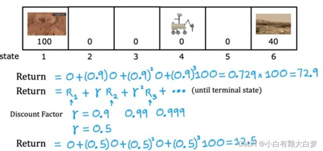
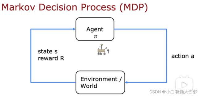
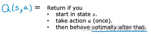
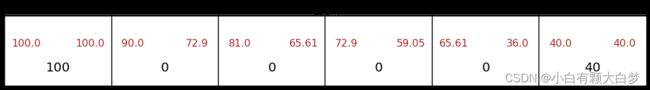
- 深度 Qlearning:在直播推荐系统中的应用
AGI通用人工智能之禅
程序员提升自我硅基计算碳基计算认知计算生物计算深度学习神经网络大数据AIGCAGILLMJavaPython架构设计Agent程序员实现财富自由
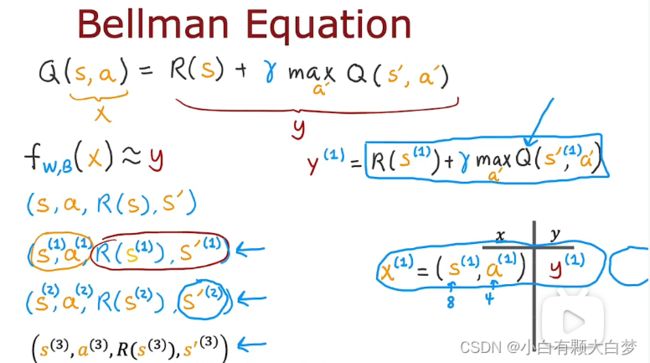
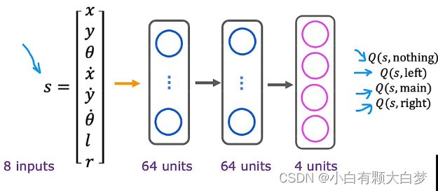
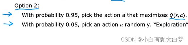
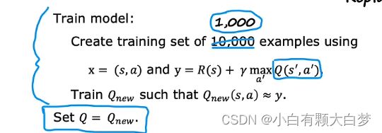
深度Q-learning:在直播推荐系统中的应用关键词:深度Q-learning,强化学习,直播推荐系统,个性化推荐1.背景介绍1.1问题的由来随着互联网技术的飞速发展,直播平台如雨后春笋般涌现。面对海量的直播内容,用户很难快速找到自己感兴趣的内容。因此,个性化推荐系统在直播平台中扮演着越来越重要的角色。1.2研究现状目前,主流的个性化推荐算法包括协同过滤、基于内容的推荐等。这些方法在一定程度上缓
- 未来软件市场是怎么样的?做开发的生存空间如何?
cesske
软件需求
目录前言一、未来软件市场的发展趋势二、软件开发人员的生存空间前言未来软件市场是怎么样的?做开发的生存空间如何?一、未来软件市场的发展趋势技术趋势:人工智能与机器学习:随着技术的不断成熟,人工智能将在更多领域得到应用,如智能客服、自动驾驶、智能制造等,这将极大地推动软件市场的增长。云计算与大数据:云计算服务将继续普及,大数据技术的应用也将更加广泛。企业将更加依赖云计算和大数据来优化运营、提升效率,并
- 个人学习笔记7-6:动手学深度学习pytorch版-李沐
浪子L
深度学习深度学习笔记计算机视觉python人工智能神经网络pytorch
#人工智能##深度学习##语义分割##计算机视觉##神经网络#计算机视觉13.11全卷积网络全卷积网络(fullyconvolutionalnetwork,FCN)采用卷积神经网络实现了从图像像素到像素类别的变换。引入l转置卷积(transposedconvolution)实现的,输出的类别预测与输入图像在像素级别上具有一一对应关系:通道维的输出即该位置对应像素的类别预测。13.11.1构造模型下
- Rust 所有权 简介
东离与糖宝
rust后端rust开发语言
文章目录发现宝藏1.所有权基本概念2.所有权规则3.变量作用域4.栈与堆4.1栈(Stack)4.2堆(Heap)5.String类型5.1String类型5.2String的内存分配5.3所有权与内存管理5.4String与切片6.变量与数据交互方式6.1移动(Move)6.2.克隆(Clone)7.所有权与函数7.1.传递参数7.2.返回值总结发现宝藏前些天发现了一个巨牛的人工智能学习网站,通
- python中zeros用法_Python中的numpy.zeros()用法
江平舟
python中zeros用法
numpy.zeros()函数是最重要的函数之一,广泛用于机器学习程序中。此函数用于生成包含零的数组。numpy.zeros()函数提供给定形状和类型的新数组,并用零填充。句法numpy.zeros(shape,dtype=float,order='C'参数形状:整数或整数元组此参数用于定义数组的尺寸。此参数用于我们要在其中创建数组的形状,例如(3,2)或2。dtype:数据类型(可选)此参数用于
- 【NumPy】深入解析numpy.zeros()函数
二七830
numpy
欢迎莅临我的个人主页这里是我深耕Python编程、机器学习和自然语言处理(NLP)领域,并乐于分享知识与经验的小天地!博主简介:我是二七830,一名对技术充满热情的探索者。多年的Python编程和机器学习实践,使我深入理解了这些技术的核心原理,并能够在实际项目中灵活应用。尤其是在NLP领域,我积累了丰富的经验,能够处理各种复杂的自然语言任务。技术专长:我熟练掌握Python编程语言,并深入研究了机
- 【中国国际航空-注册_登录安全分析报告】
风控牛
验证码接口安全评测系列安全行为验证极验网易易盾智能手机
前言由于网站注册入口容易被黑客攻击,存在如下安全问题:1.暴力破解密码,造成用户信息泄露2.短信盗刷的安全问题,影响业务及导致用户投诉3.带来经济损失,尤其是后付费客户,风险巨大,造成亏损无底洞所以大部分网站及App都采取图形验证码或滑动验证码等交互解决方案,但在机器学习能力提高的当下,连百度这样的大厂都遭受攻击导致点名批评,图形验证及交互验证方式的安全性到底如何?请看具体分析一、中国国际航空PC
- 机器学习 流形数据降维:UMAP 降维算法
小嗷犬
Python机器学习#数据分析及可视化机器学习算法人工智能
✅作者简介:人工智能专业本科在读,喜欢计算机与编程,写博客记录自己的学习历程。个人主页:小嗷犬的个人主页个人网站:小嗷犬的技术小站个人信条:为天地立心,为生民立命,为往圣继绝学,为万世开太平。本文目录UMAP简介理论基础特点与优势应用场景在Python中使用UMAP安装umap-learn库使用UMAP可视化手写数字数据集UMAP简介UMAP(UniformManifoldApproximatio
- 七.正则化
愿风去了
吴恩达机器学习之正则化(Regularization)http://www.cnblogs.com/jianxinzhou/p/4083921.html从数学公式上理解L1和L2https://blog.csdn.net/b876144622/article/details/81276818虽然在线性回归中加入基函数会使模型更加灵活,但是很容易引起数据的过拟合。例如将数据投影到30维的基函数上,模
- 管理员权限的软件不能开机自启动的解决方法
ss_ctrl
这是几种解决方法:1.将启动参数写入到32位注册表里面去在64位系统下我们64位的程序访问此HKEY_LOCAL_MACHINE\SOFTWARE\Microsoft\Windows\CurrentVersion\Run注册表路径,是可以正确访问的,32位程序访问此注册表路径时,默认会被系统自动映射到HKEY_LOCAL_MACHINE\SOFTWARE\WOW6432Node\Microsoft
- 机器学习-------数据标准化
罔闻_spider
数据分析算法机器学习人工智能
什么是归一化,它与标准化的区别是什么?一作用在做训练时,需要先将特征值与标签标准化,可以防止梯度防炸和过拟合;将标签标准化后,网络预测出的数据是符合标准正态分布的—StandarScaler(),与真实值有很大差别。因为StandarScaler()对数据的处理是(真实值-平均值)/标准差。同时在做预测时需要将输出数据逆标准化提升模型精度:标准化/归一化使不同维度的特征在数值上更具比较性,提高分类
- ztree设置禁用节点
3213213333332132
JavaScriptztreejsonsetDisabledNodeAjax
ztree设置禁用节点的时候注意,当使用ajax后台请求数据,必须要设置为同步获取数据,否者会获取不到节点对象,导致设置禁用没有效果。
$(function(){
showTree();
setDisabledNode();
});
- JVM patch by Taobao
bookjovi
javaHotSpot
在网上无意中看到淘宝提交的hotspot patch,共四个,有意思,记录一下。
7050685:jsdbproc64.sh has a typo in the package name
7058036:FieldsAllocationStyle=2 does not work in 32-bit VM
7060619:C1 should respect inline and
- 将session存储到数据库中
dcj3sjt126com
sqlPHPsession
CREATE TABLE sessions (
id CHAR(32) NOT NULL,
data TEXT,
last_accessed TIMESTAMP NOT NULL,
PRIMARY KEY (id)
);
<?php
/**
* Created by PhpStorm.
* User: michaeldu
* Date
- Vector
171815164
vector
public Vector<CartProduct> delCart(Vector<CartProduct> cart, String id) {
for (int i = 0; i < cart.size(); i++) {
if (cart.get(i).getId().equals(id)) {
cart.remove(i);
- 各连接池配置参数比较
g21121
连接池
排版真心费劲,大家凑合看下吧,见谅~
Druid
DBCP
C3P0
Proxool
数据库用户名称 Username Username User
数据库密码 Password Password Password
驱动名
- [简单]mybatis insert语句添加动态字段
53873039oycg
mybatis
mysql数据库,id自增,配置如下:
<insert id="saveTestTb" useGeneratedKeys="true" keyProperty="id"
parameterType=&
- struts2拦截器配置
云端月影
struts2拦截器
struts2拦截器interceptor的三种配置方法
方法1. 普通配置法
<struts>
<package name="struts2" extends="struts-default">
&
- IE中页面不居中,火狐谷歌等正常
aijuans
IE中页面不居中
问题是首页在火狐、谷歌、所有IE中正常显示,列表页的页面在火狐谷歌中正常,在IE6、7、8中都不中,觉得可能那个地方设置的让IE系列都不认识,仔细查看后发现,列表页中没写HTML模板部分没有添加DTD定义,就是<!DOCTYPE html PUBLIC "-//W3C//DTD XHTML 1.0 Transitional//EN" "http://www.w3
- String,int,Integer,char 几个类型常见转换
antonyup_2006
htmlsql.net
如何将字串 String 转换成整数 int?
int i = Integer.valueOf(my_str).intValue();
int i=Integer.parseInt(str);
如何将字串 String 转换成Integer ?
Integer integer=Integer.valueOf(str);
如何将整数 int 转换成字串 String ?
1.
- PL/SQL的游标类型
百合不是茶
显示游标(静态游标)隐式游标游标的更新和删除%rowtyperef游标(动态游标)
游标是oracle中的一个结果集,用于存放查询的结果;
PL/SQL中游标的声明;
1,声明游标
2,打开游标(默认是关闭的);
3,提取数据
4,关闭游标
注意的要点:游标必须声明在declare中,使用open打开游标,fetch取游标中的数据,close关闭游标
隐式游标:主要是对DML数据的操作隐
- JUnit4中@AfterClass @BeforeClass @after @before的区别对比
bijian1013
JUnit4单元测试
一.基础知识
JUnit4使用Java5中的注解(annotation),以下是JUnit4常用的几个annotation: @Before:初始化方法 对于每一个测试方法都要执行一次(注意与BeforeClass区别,后者是对于所有方法执行一次)@After:释放资源 对于每一个测试方法都要执行一次(注意与AfterClass区别,后者是对于所有方法执行一次
- 精通Oracle10编程SQL(12)开发包
bijian1013
oracle数据库plsql
/*
*开发包
*包用于逻辑组合相关的PL/SQL类型(例如TABLE类型和RECORD类型)、PL/SQL项(例如游标和游标变量)和PL/SQL子程序(例如过程和函数)
*/
--包用于逻辑组合相关的PL/SQL类型、项和子程序,它由包规范和包体两部分组成
--建立包规范:包规范实际是包与应用程序之间的接口,它用于定义包的公用组件,包括常量、变量、游标、过程和函数等
--在包规
- 【EhCache二】ehcache.xml配置详解
bit1129
ehcache.xml
在ehcache官网上找了多次,终于找到ehcache.xml配置元素和属性的含义说明文档了,这个文档包含在ehcache.xml的注释中!
ehcache.xml : http://ehcache.org/ehcache.xml
ehcache.xsd : http://ehcache.org/ehcache.xsd
ehcache配置文件的根元素是ehcahe
ehcac
- java.lang.ClassNotFoundException: org.springframework.web.context.ContextLoaderL
白糖_
javaeclipsespringtomcatWeb
今天学习spring+cxf的时候遇到一个问题:在web.xml中配置了spring的上下文监听器:
<listener>
<listener-class>org.springframework.web.context.ContextLoaderListener</listener-class>
</listener>
随后启动
- angular.element
boyitech
AngularJSAngularJS APIangular.element
angular.element
描述: 包裹着一部分DOM element或者是HTML字符串,把它作为一个jQuery元素来处理。(类似于jQuery的选择器啦) 如果jQuery被引入了,则angular.element就可以看作是jQuery选择器,选择的对象可以使用jQuery的函数;如果jQuery不可用,angular.e
- java-给定两个已排序序列,找出共同的元素。
bylijinnan
java
import java.util.ArrayList;
import java.util.Arrays;
import java.util.List;
public class CommonItemInTwoSortedArray {
/**
* 题目:给定两个已排序序列,找出共同的元素。
* 1.定义两个指针分别指向序列的开始。
* 如果指向的两个元素
- sftp 异常,有遇到的吗?求解
Chen.H
javajcraftauthjschjschexception
com.jcraft.jsch.JSchException: Auth cancel
at com.jcraft.jsch.Session.connect(Session.java:460)
at com.jcraft.jsch.Session.connect(Session.java:154)
at cn.vivame.util.ftp.SftpServerAccess.connec
- [生物智能与人工智能]神经元中的电化学结构代表什么?
comsci
人工智能
我这里做一个大胆的猜想,生物神经网络中的神经元中包含着一些化学和类似电路的结构,这些结构通常用来扮演类似我们在拓扑分析系统中的节点嵌入方程一样,使得我们的神经网络产生智能判断的能力,而这些嵌入到节点中的方程同时也扮演着"经验"的角色....
我们可以尝试一下...在某些神经
- 通过LAC和CID获取经纬度信息
dai_lm
laccid
方法1:
用浏览器打开http://www.minigps.net/cellsearch.html,然后输入lac和cid信息(mcc和mnc可以填0),如果数据正确就可以获得相应的经纬度
方法2:
发送HTTP请求到http://www.open-electronics.org/celltrack/cell.php?hex=0&lac=<lac>&cid=&
- JAVA的困难分析
datamachine
java
前段时间转了一篇SQL的文章(http://datamachine.iteye.com/blog/1971896),文章不复杂,但思想深刻,就顺便思考了一下java的不足,当砖头丢出来,希望引点和田玉。
-----------------------------------------------------------------------------------------
- 小学5年级英语单词背诵第二课
dcj3sjt126com
englishword
money 钱
paper 纸
speak 讲,说
tell 告诉
remember 记得,想起
knock 敲,击,打
question 问题
number 数字,号码
learn 学会,学习
street 街道
carry 搬运,携带
send 发送,邮寄,发射
must 必须
light 灯,光线,轻的
front
- linux下面没有tree命令
dcj3sjt126com
linux
centos p安装
yum -y install tree
mac os安装
brew install tree
首先来看tree的用法
tree 中文解释:tree
功能说明:以树状图列出目录的内容。
语 法:tree [-aACdDfFgilnNpqstux][-I <范本样式>][-P <范本样式
- Map迭代方式,Map迭代,Map循环
蕃薯耀
Map循环Map迭代Map迭代方式
Map迭代方式,Map迭代,Map循环
>>>>>>>>>>>>>>>>>>>>>>>>>>>>>>>>>>>>>>>>
蕃薯耀 2015年
- Spring Cache注解+Redis
hanqunfeng
spring
Spring3.1 Cache注解
依赖jar包:
<!-- redis -->
<dependency>
<groupId>org.springframework.data</groupId>
<artifactId>spring-data-redis</artifactId>
- Guava中针对集合的 filter和过滤功能
jackyrong
filter
在guava库中,自带了过滤器(filter)的功能,可以用来对collection 进行过滤,先看例子:
@Test
public void whenFilterWithIterables_thenFiltered() {
List<String> names = Lists.newArrayList("John"
- 学习编程那点事
lampcy
编程androidPHPhtml5
一年前的夏天,我还在纠结要不要改行,要不要去学php?能学到真本事吗?改行能成功吗?太多的问题,我终于不顾一切,下定决心,辞去了工作,来到传说中的帝都。老师给的乘车方式还算有效,很顺利的就到了学校,赶巧了,正好学校搬到了新校区。先安顿了下来,过了个轻松的周末,第一次到帝都,逛逛吧!
接下来的周一,是我噩梦的开始,学习内容对我这个零基础的人来说,除了勉强完成老师布置的作业外,我已经没有时间和精力去
- 架构师之流处理---------bytebuffer的mark,limit和flip
nannan408
ByteBuffer
1.前言。
如题,limit其实就是可以读取的字节长度的意思,flip是清空的意思,mark是标记的意思 。
2.例子.
例子代码:
String str = "helloWorld";
ByteBuffer buff = ByteBuffer.wrap(str.getBytes());
Sy
- org.apache.el.parser.ParseException: Encountered " ":" ": "" at line 1, column 1
Everyday都不同
$转义el表达式
最近在做Highcharts的过程中,在写js时,出现了以下异常:
严重: Servlet.service() for servlet jsp threw exception
org.apache.el.parser.ParseException: Encountered " ":" ": "" at line 1,
- 用Java实现发送邮件到163
tntxia
java实现
/*
在java版经常看到有人问如何用javamail发送邮件?如何接收邮件?如何访问多个文件夹等。问题零散,而历史的回复早已经淹没在问题的海洋之中。
本人之前所做过一个java项目,其中包含有WebMail功能,当初为用java实现而对javamail摸索了一段时间,总算有点收获。看到论坛中的经常有此方面的问题,因此把我的一些经验帖出来,希望对大家有些帮助。
此篇仅介绍用
- 探索实体类存在的真正意义
java小叶檀
POJO
一. 实体类简述
实体类其实就是俗称的POJO,这种类一般不实现特殊框架下的接口,在程序中仅作为数据容器用来持久化存储数据用的
POJO(Plain Old Java Objects)简单的Java对象
它的一般格式就是
public class A{
private String id;
public Str