论文笔记 Weakly Supervised Deep Detection Networks - CVPR 2016

Weakly Supervised Deep Detection Networks

Hakan Bilen, Andrea Vedaldi CVPR, 2016 (PDF) (Citations 581)

Abstract

优点

提出了一种弱监督深度检测架构，该架构使用图像级图片，同时执行区域选择和分类。

在 PASCAL VOC 数据上隐式学习优于其他弱监督检测系统的目标检测器。

该模型是一个端到端架构，在图像级分类任务方面的表现优于标准数据增强和微调技术。

缺点

该架构无法检测具有多个同类别物体的图片。华中科技大学的 Peng Tang 等人在 CVPR(2017) 提出 OICR 改善了 WSDDN 的性能，但是同样没有解决这个问题。东京大学的 Kosugi 等人在 ICCV(2019) 提出了 CAP 和 SRN 两种标签，利用空间限制解决了在一张图片上无法检测具有多个同类别物体的问题。

1. Introduction

由于预训练的 CNN 可以很好地泛化到大量任务，它们应该包含有意义的数据表示，WSDDN正是基于这个假设提出的。其网络架构如下图所示：

图1. WSDDN 网络架构

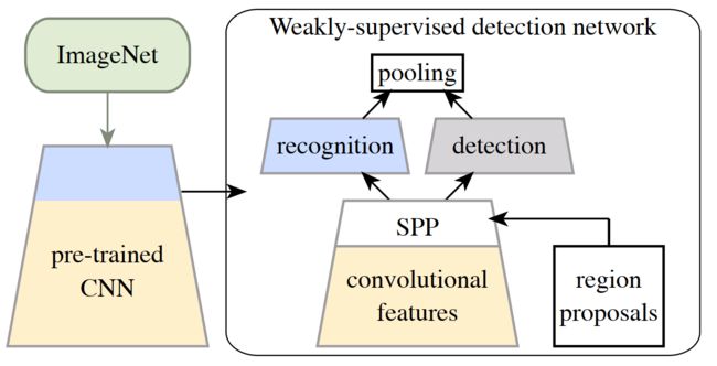
首先在ImageNet数据集上预训练CNN，输入图片经过预训练的CNN获得Feature Map和Region Proposal获得建议区域，所获得的Feature Map和Region Proposal经过SPP池化获得区域特征向量。然后对获得的区域特征向量进行分流（分类流和检测流），最后在通过聚合操作获取区域得分，对所有区域的识别和检测分数进行分类，来预测整个图像的类别，然后在学习过程中注入图像级监督。此处参见了2017CVPR提出的OICR网络架构和2019ICCV提出的CAP和SRN标注。

图2. OICR 网络架构

图3. Kosugi 等人提出的 CAP 和 SRN 标注

作者将此方法与多实例学习（MIL）进行比较。 MIL 在选择图像中的哪些区域看起来像感兴趣的对象和使用所选区域估计对象的外观模型之间交替进行。因此，MIL 使用外观模型本身来执行区域选择。我们的技术在根本上与 MIL 不同，因为区域是由网络中的专用并行检测分支选择的，该分支独立于识别分支。通过这种方式，我们的方法有助于避免 MIL 的缺陷之一，即该方法陷入局部最优的趋势。（对于该处，个人对周志华[5]的综述中inexact supervision的理解，作者想表达的是WSDDN与交替学习方法的对比，而非MIL的对比。图2将可以使用WSDDN的多实例检测网络MIDN视为MIL，根据OICR论文的观点，该方法应认识属于MIL范畴。）

2. Related Work

大多数现有的 WSD 方法将此任务表述为 MIL。在这个MIL中，图像被解释为多个区域组成的bag。如果图像被标记为正，则假设其中一个区域紧密包含感兴趣的对象。如果图像被标记为负，则没有区域包含该对象。学习在估计对象外观模型和使用外观模型选择正包中的哪些区域对应于对象之间交替进行。MIL 策略导致非凸优化问题；在实践中，求解器往往会陷入局部最优解，因此解的质量很大程度上取决于初始化。Several papers have focused on developing various initialization strategies and on regularizing the optimization problem. WSD的另一个研究方向是基于识别图像部件之间的相似性的想法。

3. Method

图4. The figure illustrates the architecture of WSDDN.

总体思路

• Pre-trained CNN
• construct the WSDDN as an architectural modification of this CNN
• train/fine-tune the WSDDN on a target dataset, once more using only image-level annotations

3.1. Pre-trained network

3.2. Weakly supervised deep detection network

首先，将紧跟在最后一个卷积块的ReLU层（relu5）之后的最后一个池化层（pool5）替换为实现SPP池化层。以图像$x$和区域（边界框）$R$作为输入，并产生一个特征向量$\varphi (x;R)$作为输出：

$$\varphi (\mathbf{x};R)={\varphi }_{\mathrm{S}\mathrm{P}\mathrm{P}}(\cdot ;R)\circ {\varphi }_{\mathrm{r}\mathrm{e}\mathrm{l}\mathrm{u}5}(\mathbf{x})$$

注意到，${\varphi }_{\mathrm{r}\mathrm{e}\mathrm{l}\mathrm{u}5}$只需要对整个图像计算一次，$\varphi (\mathbf{x};R)$对于任何给定区域$R$计算都很快。

在实践中，修改SPP层，使其不接受单个区域，而是接受完整的候选区域列表$R$；$\varphi (x;R)=\varphi (x;R_1),\dots ,\varphi (x;R_n)$变成四维，因为原单独$\varphi (x;R)$是$3DTensor$）。

而后，$\varphi (x;R)$经过${\varphi }_{\mathrm{f}\mathrm{c}6}$和${\varphi }_{\mathrm{f}\mathrm{c}7}$得到区域Proposal feature vector，进而分为分类流和检测流。

• Proposal feature vector 经过FC层分别得到 ${\mathbf{x}}^c，{\mathbf{x}}^d\in {\mathbb{R}}^{C\times |R|}$
• 分类流，${\mathbf{x}}^c$经过Sofrmax层得到${\left[{\sigma }_{class}\left({\mathbf{x}}^c\right)\right]}_{ij}=\frac{e^{x_{ij}^c}}{{\sum }_{k=1}^C{e}^{x_{kj}^c}}$, 表示建议区域$j$属于类别$i$的概率。
• 检测流，${\mathbf{x}}^d$经过Sofrmax层得到${\left[{\sigma }_{det}\left({\mathbf{x}}^d\right)\right]}_{ij}=\frac{e^{x_{ij}^c}}{{\sum }_{k=1}^{|R|}{e}^{x_{ik}^c}}$, 表示图片被分类为$i$类时建议区域$j$作的贡献。
• Combined region scores and detection，初始建议得分矩阵${\mathbf{x}}^R=\sigma \left({\mathbf{x}}^c\right)\odot \sigma \left({\mathbf{x}}^d\right)$，其中每个元素 $x_{ij}^R$ 表示建议区域 $r_j$ 对类别$i$的得分，然后进行区域得分排序，执行非极大值抑制（NMS），只留下可能性最大的区域。
• Image-level classification scores，对所有区域建议求和得到图像分类得分$y_c={\sum }_{r=1}^{|R|}{x}_{cr}^R$，表示图像对类别$c$的得分。

3.3. Training WSDDN

损失函数：
$$E(\mathbf{w})=\frac{\lambda }{2}\Vert \mathbf{w}{\Vert }^2+\sum _{i=1}^n\sum _{k=1}^C\log \left(y_{ki}\left({\varphi }_k^{\mathbf{y}}\left({\mathbf{x}}_i\mid \mathbf{w}\right)-\frac{1}{2}\right)+\frac{1}{2}\right)$$

The data is a collection of images $x_i,i=1,\dots ,n$ with image level labels $y_i\in {-1,1}^C$. As ${\varphi }_k^{\mathbf{y}}\left({\mathbf{x}}_i\mid \mathbf{w}\right)$ is in range of $(0,1)$, it can be considered as a probability of class $k$ being present in image $x_i$, i.e. $p(y_{ki}=1)$. When the ground-truth label is positive, the binary log loss becomes $log(p(y_{ki}=1))$, $log(1-p(y_{ki}=1))$ otherwise.

3.4. Spatial Regulariser

As WSDDN is optimised for image-level class labels, it does not guarantee any spatial smoothness such that if a region obtains a high score for an object class, the neighbouring regions with high overlap will also have high scores. In the supervised detection case, Fast R-CNN takes the region proposals that have IoU with a ground truth box of at least 50% as positive samples and learns to regress them into their corresponding ground truth bounding box. As our method does not have access to ground truth boxes, we follow a soft regularisation strategy that penalises the feature map discrepancies between the highest scoring region and the regions with at least 60% IoU during training: (此处空间正则化项参照博文进行了修改)

$$\frac{1}{nC}\sum _{k=1}^C\frac{1}{2}{\varphi }_k^{\mathbf{y}}\left({\mathbf{x}}_i\mid \mathbf{w}\right)\sum _{i=1}^{n_k^{+}}{\left({\varphi }_{kp}^{\mathrm{f}\mathrm{c}7}-{\varphi }_{ki}^{\mathrm{f}\mathrm{c}7}\right)}^{\mathrm{T}}\left({\varphi }_{kp}^{\mathrm{f}\mathrm{c}7}-{\varphi }_{ki}^{\mathrm{f}\mathrm{c}7}\right)$$

where $n_k^{+}$ is the number of positive images for the class $k$ and $kp={\text{arg max}}_j{\varphi }_{kj}^y$ is the highest scoring region in image $i$ for the class $k$. We add this regularisation term to the cost function in $eq.(3)$.

综上所述，即最终损失函数为：
$$E(\mathbf{w})=\frac{\lambda }{2}\Vert \mathbf{w}{\Vert }^2+\sum _{i=1}^n\sum _{k=1}^C\log \left(y_{ki}\left({\varphi }_k^{\mathbf{y}}\left({\mathbf{x}}_i\mid \mathbf{w}\right)-\frac{1}{2}\right)+\frac{1}{2}\right)+\frac{1}{nC}\sum _{k=1}^C\frac{1}{2}{\varphi }_k^{\mathbf{y}}\left({\mathbf{x}}_i\mid \mathbf{w}\right)\sum _{i=1}^{n_k^{+}}{\left({\varphi }_{kp}^{\mathrm{f}\mathrm{c}7}-{\varphi }_{ki}^{\mathrm{f}\mathrm{c}7}\right)}^{\mathrm{T}}\left({\varphi }_{kp}^{\mathrm{f}\mathrm{c}7}-{\varphi }_{ki}^{\mathrm{f}\mathrm{c}7}\right)$$

延申阅读

[1] B. Zhou, A. Khosla, A. Lapedriza, A. Oliva, and A. Torralba. Object detectors emerge in deep scene CNNs. In ICLR, 2015.

[2] T. G. Dietterich, R. H. Lathrop, and T. Lozano-Pérez. Solving the multiple instance problem with axis-parallel rectangles. Artificial intelligence, 89(1):31–71, 1997.

[3] Tang P , Wang X , Bai X , et al. Multiple Instance Detection Network with Online Instance Classifier Refinement[J]. IEEE Conference on Computer Vision & Pattern Recognition, 2017.

[4] Kosugi S , Yamasaki T , Aizawa K . Object-Aware Instance Labeling for Weakly Supervised Object Detection[J]. 2019.

[5] Zhou Z H. A brief introduction to weakly supervised learning[J]. National science review, 2018, 5(1): 44-53.