Learning machine learning algorithm(一)

机器学习——逻辑回归

Problem 1：如何理解coef_和intercept_两个模型参数

Solution 1：对于线性回归和逻辑回归，其目标函数为：f(x) =w0+w1x1+wxx2+…
如果有激活函数sigmoid，增加非线性变化，则为分类即逻辑回归；如果没有激活函数，则为线性回归。而对于coef_和intercept两个模型参数，常做如下用法

lr = LogisticRegression()
lr.coef_        #除w0外的其余wi
lr.intercept_   #w0

---

Problem 2：如何利用matplotlib库绘制散点图

Solution 2：常调用scatter()函数，具体使用方法及参数说明参见：https://blog.csdn.net/xiaobaicai4552/article/details/79065990
补充：scatter()函数 c（color）参数的使用:以上述代码为例：设置c = y_label，而y_label有两类值即0/1，且与x_label中的数对相对应，也就是说一对一的逻辑关系，用0/1两类值代表两类颜色来区分点。更一步说，只需要y_label中存在任意不相等的2对数即可，例如：
设置y_label = np.array([1,1,1,2,2,2])也可达到相同的区分效果

---

Problem 3：对于scatter()函数中x_features[:,0]和x_features[:,1]的设置不太清晰

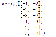
Solution 3：x_features = np.array([[-1, -2], [-2, -1], [-3, -2], [1, 3], [2, 1], [3, 2]]) 即如图所示：

x_features[:,0]则代表二元数对中的第一元的集合，x_features[:,1]代表二元数对中的第二元的集合

---

Problem 4：对plt.xlim()和plt.ylim()理解模糊

Solution 4：xlim()/ylim()两函数的功能是设置x/y轴的数据显示范围，或者调用两函数来获取对应轴上数据的最大最小值（范围），使用方法如下（以设置x轴为例，y轴同理）：

plt.xlim(xmin,xmax)   #xmin为x轴上的最小值，xmax为x轴上的最大值
xmin,xmax = plt.xlim()

---

Problem 5：不了解Numpy中的meshgrid()函数

Solution 5：从坐标向量中返回坐标矩阵，简而言之，就是一维向量和另一维向量之间的数进行组合（先后顺序不可颠倒），获得一个由二元数对组成的二维矩阵，返回两个数组(x/y)
参见：https://blog.csdn.net/littlehaes/article/details/83543459

---

Problem 6：不了解Numpy中的linspace()函数

Solution 6：该函数的功能是在指定的间隔内返回均匀间隔的数字
参见：https://blog.csdn.net/Dontla/article/details/98342415

---

Problem 7：predict_proba()和predict()两函数的作用和区别

Solution 7:参见：https://www.cnblogs.com/mrtop/p/10309083.html

---

Problem 8：Numpy中的np.c_[]和np.r_[]的作用和区别

Solution 8:两方法均用于连接矩阵，区别在于np.r_按行叠加矩阵，np.c_按列叠加矩阵
参见：https://blog.csdn.net/C_chuxin/article/details/84777481

---

Problem 9：Numpy中的扁平化函数ravel()的使用和拓展

Solution 9:Numpy提供了两个扁平化函数：ravel和flatten()函数，这两个函数实现的功能相同，但在内存上有一些差别
参见：https://www.cnblogs.com/mzct123/p/8659193.html

---

Problem 10：关于Numpy中的reshape()函数

Solution 10：reshape()函数的功能是在不改变矩阵数值的前提下修改矩阵的形状
可参见：https://blog.csdn.net/qq_28618765/article/details/78083895?utm_medium=distribute.pc_relevant.none-task-blog-BlogCommendFromMachineLearnPai2-1.add_param_isCf&depth_1-utm_source=distribute.pc_relevant.none-task-blog-BlogCommendFromMachineLearnPai2-1.add_param_isCf
拓展:Numpy中类似的还有tranpose()函数，关于tranpose()函数可参见：https://blog.csdn.net/u012762410/article/details/78912667

---

Problem 11：关于plt.contour的理解应用及其相关拓展

Solution 11:参见两篇博客：https://www.cnblogs.com/nxf-rabbit75/p/10463093.html
https://blog.csdn.net/lanchunhui/article/details/70495353

---

基于鸢尾花(iris)数据集的逻辑回归实践

Step 1：函数库导入

##  基础函数库
import numpy as np 
import pandas as pd

## 绘图函数库
import matplotlib.pyplot as plt
import seaborn as sns

Step 2：数据读取/载入

##利用sklearn中自带的iris数据作为数据载入，并利用Pandas转化为DataFrame格式
from sklearn.datasets import load_iris
data = load_iris() 
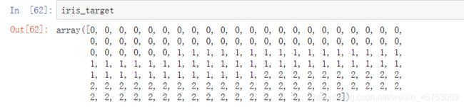
iris_target = data.target      #得到数据对应的标签,已经过处理，iris_target里的0/1/2分别代表三种类型的花
iris_attributes = data.data    #获取属性数据
labels = data.feature_names    #获取属性值
##利用Pandas转化为DataFrame格式
iris_features = pd.DataFrame(data=iris_attributes, columns=labels)  

step 3：查看数据信息

iris_features.info() #利用info()查看数据的整体信息
iris_features.head()
##iris_features.tail()
iris_features.describe()

step 4：数据可视化

## 合并标签和特征信息
iris_all = iris_features.copy() #进行浅拷贝，防止对于原始数据的修改
iris_all['target'] = iris_target 
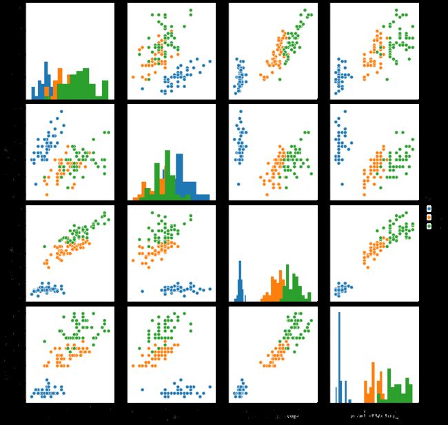
## 特征与标签组合的散点可视化
sns.pairplot(data=iris_all,diag_kind='hist', hue= 'target')
plt.show()

##绘制箱线图
for col in iris_features.columns:
    sns.boxplot(x='target', y=col, saturation=0.5, 
palette='pastel', data=iris_all)
    plt.title(col)
    plt.show()

step 5：利用逻辑回归模型在二分类上进行训练和预测

##为了正确评估模型性能，将数据划分为训练集和测试集，并在训练集上训练模型，在测试集上验证模型性能。
from sklearn.model_selection import train_test_split
##选择其类别为0和1的样本（不包括类别为2的样本）
iris_features_part=iris_features.iloc[:100]
iris_target_part=iris_target[:100]
##测试集大小为20%，80%/20%分
x_train,x_test,y_train,y_test=train_test_split(iris_features_part,iris_target_part,test_size=0.2,random_state=2020)
##从sklearn中导入逻辑回归模型
from sklearn.linear_model import LogisticRegression
##定义逻辑回归模型
clf=LogisticRegression(random_state=0,solver='lbfgs')
##在训练集上训练逻辑回归模型
clf.fit(x_train,y_train)
##查看其对应的w
print('the weight of Logistic Regression:',clf.coef_)

##查看其对应的w0
print('the intercept(w0) of Logistic Regression:',clf.intercept_)

##在训练集和测试集上分布利用训练好的模型进行预测
train_predict=clf.predict(x_train)
test_predict=clf.predict(x_test)

step 6：模型评估

from sklearn import metrics
##利用accuracy（准确度）【预测正确的样本数目占总预测样本数目的比例】评估模型效果
print('The accuracy of the Logistic Regression is:',metrics.accuracy_score(y_train,train_predict))
print('The accuracy of the Logistic Regression is:',metrics.accuracy_score(y_test,test_predict))

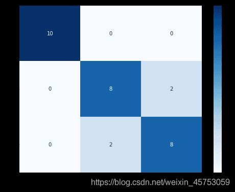
##查看混淆矩阵(预测值和真实值的各类情况统计矩阵)
confusion_matrix_result=metrics.confusion_matrix(test_predict,y_test)
print('The confusion matrix result:\n',confusion_matrix_result)

##利用热力图对于结果进行可视化
plt.figure(figsize=(8,6))
sns.heatmap(confusion_matrix_result,annot=True,cmap='Blues')
plt.xlabel('Predictedlabels')
plt.ylabel('Truelabels')
plt.show()

step 7：利用逻辑回归模型在三分类(多分类)上进行训练和预测

##测试集大小为20%，80%/20%分
x_train,x_test,y_train,y_test=train_test_split(iris_features,iris_target,test_size=0.2,random_state=2020)
##定义逻辑回归模型
clf=LogisticRegression(random_state=0,solver='lbfgs')
##在训练集上训练逻辑回归模型
clf.fit(x_train,y_train)
##查看其对应的w
print('the weight of Logistic Regression:\n',clf.coef_)
##查看其对应的w0
print('the intercept(w0) of Logistic Regression:\n',clf.intercept_)
##由于这个是3分类，所有我们这里得到了三个逻辑回归模型的参数，其三个逻辑回归组合起来即可实现三分类
##在训练集和测试集上分布利用训练好的模型进行预测
train_predict=clf.predict(x_train)
test_predict=clf.predict(x_test)
##由于逻辑回归模型是概率预测模型（前文介绍的p=p(y=1|x,\theta)）,所有我们可以利用predict_proba函数预测其概率

train_predict_proba=clf.predict_proba(x_train)
test_predict_proba=clf.predict_proba(x_test)

step 8：模型评估

print('The test predict Probability of each class:\n',test_predict_proba)
##其中第一列代表预测为0类的概率，第二列代表预测为1类的概率，第三列代表预测为2类的概率。

##利用accuracy（准确度）【预测正确的样本数目占总预测样本数目的比例】评估模型效果
print('The accuracy of the Logistic Regression is:',metrics.accuracy_score(y_train,train_predict))
print('The accuracy of the Logistic Regression is:',metrics.accuracy_score(y_test,test_predict))
##查看混淆矩阵
confusion_matrix_result=metrics.confusion_matrix(test_predict,y_test)
print('The confusion matrix result:\n',confusion_matrix_result)

##利用热力图对于结果进行可视化
plt.figure(figsize=(8,6))
sns.heatmap(confusion_matrix_result,annot=True,cmap='Blues')
plt.xlabel('Predicted labels')
plt.ylabel('True labels')
plt.show()

代码参考：https://developer.aliyun.com/ai/scenario/9ad3416619b1423180f656d1c9ae44f7?spm=5176.12901015.0.i12901015.5589525csLKDtN

小结

关于逻辑回归算法的运用尚未学习透彻，一些知识点还未总结完，对于代码，不可仅仅停留在调库上，仅做一个调包侠。任重道远~~