paper：DeepAR: Probabilistic forecasting with autoregressive recurrent networks DeepAR模型

Deepar

Deepar与普通的时序预测模型最大的不同就在于，其预测输出的是一个概率分布，而不是一个单一的值，其假设输出是一个高斯分布

理论讲解

其也是一个encoder-decoder模型，其中encoder和decoder，encoder是一个LSTM结构，而decoder就是全连接网络

下图为网络训练的流程图

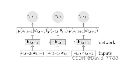
网络输入为协变量x和上一个时间步的输出z，但是注意的是，在训练的时候，z不使用上一个时间步的预测输出，而是使用真实的label值输入网络中，在 测试的时候z才使用上一个时间步的输出。

输入数据经过一个encoder得到隐藏层变量h，通过隐藏层变量经过decoder得到高斯分分布的均值和方差，通过两个全连接，注意方差通过全连接后，还有通过一个softplus的激活函数来保证方差是大于0的，根据得到的高斯分布的均值和方差建立高斯分布，然后在高斯分布中随机抽取值作为最终的预测值进行输出。

下图为网络的测试的流程图，与训练不同的就在于测试时候z使用的是上一个时间步的输出而不是真实的label

代码讲解

初始化模型参数

初始化Deepar模型的参数

class Deepar(nn.Module):
    def __init__(self,args,lstm_layers=2,dropout=0.2,pos=False):
        '''
        Args:
        :param args:已经封装好的参数，在main函数中可以查看
        :param lstm_layers: 使用多少层LSTM网络
        :param dropout:dropout率
        :param pos:在扩充时间维度时使用dropout与否
        '''
        super(Deepar, self).__init__()
        self.seq_len = args.seq_len # 已知的时间序列长度
        self.label_len = args.label_len # 为了在本任务的y中把预测部分的真实时间序列的数据拿到
        self.pred_len = args.pred_len # 需要预测的时间序列的长度
        self.d_feature = args.d_feature # 数据的维度
        self.d_model = args.d_model # embedding后的数据的维度
        self.d_ff = args.d_ff # 为lstm的hidden_size
        self.d_mark = args.d_mark # 时间维度
        self.lstm_layers = lstm_layers #使用几层的LSTM网络
        self.dropout = dropout # dropout率
        
       
        # 初始化LSTM网络
        self.lstm = nn.LSTM(input_size=self.d_model,
                            hidden_size=self.d_ff,
                            num_layers=self.lstm_layers,
                            bias=True,
                            batch_first=False,
                            dropout=self.dropout) # 初始化 LSTM网络

根据paper将LSTM的遗忘门偏置设置为1

# initialize LSTM forget gate bias to be 1 as recommanded by http://proceedings.mlr.press/v37/jozefowicz15.pdf
for names in self.lstm._all_weights:
    for name in filter(lambda n: "bias" in n, names):
        bias = getattr(self.lstm, name)
        n = bias.size(0)
        start, end = n // 4, n // 2
        bias.data[start:end].fill_(1.)

初始化激活函数，线性层和数据embedding层

self.relu = nn.ReLU()
# 输入为(batch_size,hidden_size*num_layers)-->输出为（batch_size,d_model）
self.distribution_mu = nn.Linear(self.d_ff * self.lstm_layers, self.d_model)
# 输入为(batch_size,hidden_size*num_layers)-->输出为（batch_size,d_model）
self.distribution_presigma = nn.Linear(self.d_ff * self.lstm_layers, self.d_model)
# 使用softplus激活函数 使得sigma大于0
self.distribution_sigma = nn.Softplus()
# 输入为(batch_size,d_model)-->输出为(batch_size,d_feature)
self.mu_outfc = nn.Linear(self.d_model,self.d_feature)  # 因为输入的数据经过了embedding变为d_model 现在将其降维回d_feature
# 输入为(batch_size,d_model)-->输出为(batch_size,d_feature)
self.sigma_outfc = nn.Linear(self.d_model, self.d_feature)
# 输入为（batch_size,pred_len,d_model）-->输出为（batch_size,pred_len,d_feature）
self.pred_outfc = nn.Linear(self.d_model, self.d_feature)

self.embedding = DataEmbedding_time_token(self.d_feature, self.d_mark, self.d_model)

初始化隐藏层状态和细胞状态

def init_hidden(self, input_size):
    return torch.zeros(self.params.lstm_layers, input_size, self.params.lstm_hidden_dim, device=self.params.device)

def init_cell(self, input_size):
    return torch.zeros(self.params.lstm_layers, input_size, self.params.lstm_hidden_dim, device=self.params.device)

loss 损失函数

重新定义损失函数

该损失函数是负对数损失函数，首先根据预测出来的mu，sigma，重构一个高斯分布，然后计算label在该高斯分布中的负对数似然（即在该高斯分布下的被抽中的概率），然后返回负对数似然的均值作为损失

def loss_fn(self,mu, sigma,labels): # 自定义一个负对数损失的损失函数
    '''
    Compute using gaussian the log-likehood which needs to be maximized. Ignore time steps where labels are missing.
    Args:
        mu: (Variable) dimension [batch_size] - estimated mean at time step t
        sigma: (Variable) dimension [batch_size] - estimated standard deviation at time step t
        labels: (Variable) dimension [batch_size] z_t
    Returns:
        loss: (Variable) average log-likelihood loss across the batch
    '''
    distribution = torch.distributions.normal.Normal(mu, sigma) # 利用mu,sigma重构一个高斯分布
    likelihood = distribution.log_prob(labels) # 负对数似然
    return -torch.mean(likelihood)

forward函数

处理输入数据

    def forward(self, enc_x, enc_mark, y, y_mark,mode):
        '''
        Args:
            enc_x：(batch_size,seq_len,d_feature) 已知的时间序列的数据
            enc_mark:(batch_size,seq_len,d_mark)  已知的时间序列对应的时间维度数据
            y:(batch_size,label_len+rped_len,d_feature) 包括需要预测的时间序列的数据和其前label_len的数据
            y_mark:(batch_size,label_len+pred_len,d_mark) 即y对应的时间维度的数据
            mode:判断是训练还是验证和测试
        '''
        loss = torch.zeros(1, device=enc_x.device) # 初始化loss
        B = enc_x.shape[0] # batch_size
        x_embed = self.embedding(enc_x, enc_mark)
        y_embed = self.embedding(y,y_mark) # 将时间维度和特征维度加在一起，并且embedding

使用零进行初始化需要预测的数据和输入数据

# 以下的shape (batch_size,pred_len,d_model)
pred_zero = torch.zeros_like(x_embed[:, -self.pred_len:, :]).float()
input_zero = torch.zeros_like(x_embed[:, -self.pred_len:, :]).float()

将已知的时间序列数据和使用零进行初始化的预测部分的数据拼接起来，称为x_cat_pred

将已知的时间序列和使用零进行初始化的预测部分的数据拼接起来，称为x_cat_input

虽然现在两个数据是相同的，但是x_cat_pred后面存放的是模型的预测值，而x_cat_input存放的是真实的label值

因为该模型虽然是一步一步预测，但是在训练的时候，使用的不是上一步的预测值，而是使用的是上一步预测值对应的真实的label值

x_cat_pred = torch.cat([x_embed[:, :self.seq_len, :], pred_zero], dim=1).float().to(enc_x.device) # 把初始化的预测值和原本的时序数据拼接起来，用来装预测值
x_cat_input = torch.cat([x_embed[:, :self.seq_len, :], input_zero], dim=1).float().to(enc_x.device) # 打算在训练的时候每一次输入LSTM的数据都是真实的数据，而不是上一个时间步预测值

初始化LSTM网络的隐藏层状态和细胞状态

# 初始化全零的隐藏层hidden和细胞状态cell LSTM输入需要
#并且他们的shape都是（num_layers,batch_size,d_ff）
hidden = torch.zeros(self.lstm_layers,B , self.d_ff, device=enc_x.device)
cell = torch.zeros(self.lstm_layers,B, self.d_ff, device=enc_x.device)

一次只预测已知的时间序列的下一天，因此循环pred_len次

如果是训练的时候，那么就从x_cat_input中取数据，x_cat_input中存放的是真实数据

如果不是训练的时候，那么pred_len部分的数据是未知的，因此得需要根据上一时间步预测的结果来预测下一时间步，所以就从x_cat_pred中取数据

for i in range(self.pred_len): # 因为每一次只预测下一天的时序数据 因此需要循环pred_len次
    if mode == 'train': # 如果是训练 则就使用真实的时间序列进行训练
        lstm_input = x_cat_input[:, i:i + self.seq_len, :].permute(1, 0, 2).clone()
    else: # 否则就是使用之前预测的时间序列进行训练
        lstm_input = x_cat_pred[:, i:i + self.seq_len, :].permute(1,0,2).clone()

把得到的LSTM的输入数据送入pred_onestep函数中得到预测值和mu，sigma

pred,mu,sigma = self.pred_onestep(lstm_input ,hidden,cell)

pred_onestep函数

得到输入数据，将数据送入LSTM中，得到LSTM的隐藏层状态，分别通过两个全连接神经网络，得到高斯分布的均值mu和方差sigma，其中由于方差是恒定大于0的，因此方差sigma还需要经过一个softplus激活函数来确保方差恒大于0，根据mu和sigma构建高斯分布，在高斯分布中随机抽取值作为预测值pred输出

def pred_onestep(self,x,hidden,cell):

    # 输入x是（seq_len,batch_size,self.d_feature）-->output (seq_len,batch_size,hidden_size)
    # hidden and cell (num_layers,batch_size,hidden_size)
    output, (hidden, cell) = self.lstm(x, (hidden, cell)) # (96,32,64)-->(96,32,128)
    # use h from all three layers to calculate mu and sigma
    # hidden_permute (batch_size,hidden_size*num_layers)
    hidden_permute = hidden.permute(1, 2, 0).contiguous().view(hidden.shape[1], -1)
    pre_sigma = self.distribution_presigma(hidden_permute)
    mu = self.distribution_mu(hidden_permute)
    sigma = self.distribution_sigma(pre_sigma) #使用softplus激活函数使得sigma恒大于零

    gaussian = torch.distributions.normal.Normal(mu, sigma) # 使用mu和sigma构建高斯分布的曲线
    pred = gaussian.sample()  # 预测值是在刚刚构建的高斯分布中抽样得到
    # pred and mu and sigma 都为 （batch_size,d_model）
    return pred,mu,sigma

forward函数

由于pred_onestep中得到的mu and sigma (batch_size,d_model),pred(batch_size,d_model)

因此再通过两个FC把mu and sigma -->(batch_size,d_feature)，并且sigma还多经过了一个softplus函数，来保证其恒大于0

为什么不直接在pred_onestep中把mu and sigma直接降维成d_feature呢？

因为降维成d_model是为了生成shape(batch_size,d_model)的pred，pred在后面方便可以直接加到x_cat_pred中

而由于label的shape（batch_size，d_feature），因此还需要把mu and sigam降维成（batch_size,d_feature)，才可以使得label，可以在 其产生的高斯分布中求负对数似然

其实这里也可以直接将mu and sigma (batch_size,d_feature)，然后随机在其构建的高斯分布中，随机抽取值作为pred，然后在经过相同的embedding操作得到(batch_size,d_model)的pred，在加到x_cat_pred中

# 输入为（batch_size,d_model）-->(batch_size,d_feature)
out_mu = self.mu_outfc(mu) 
# 输入sigma为（batch_size,d_model）-->(batch_size,d_feature)然后在经过一个softplus让其恒大于0，即得到out_sigma
out_sigma = self.distribution_sigma(self.sigma_outfc(sigma))

把降维成d_feature的out_mu,out_sigma和对应的真实的label送入loss_fn函数中，得到loss

# 返回lables在根据out_mu and out_sigma 构建的高斯分布曲线中的负对数似然的均值（均值是因为batch_size）
loss += self.loss_fn(out_mu,out_sigma,y[:,self.label_len+i,:])

最后再把预测的值和真实的值分别拼回两个变量中

# 然后将预测的时间序列拼接回去
x_cat_pred[:, self.seq_len + i, :] = x_cat_pred[:, self.seq_len + i, :].clone() + pred
# 把真实的label拼接回去
x_cat_input[:, self.seq_len + i, :] = x_cat_input[:, self.seq_len + i, :].clone() + y_embed[:, self.label_len + i,:]

完整的Deepar代码

import torch
import torch.nn as nn
from layers.Embed import DataEmbedding_time_token

'''
We define a recurrent network that predicts the future values of a time-dependent variable based on
past inputs and covariates.
'''
class Deepar(nn.Module):
    def __init__(self,args,lstm_layers=2,dropout=0.2,pos=False):
        '''
        Args:
        :param args:已经封装好的参数，在main函数中可以查看
        :param lstm_layers: 使用多少层LSTM网络
        :param dropout:dropout率
        :param pos:在扩充时间维度时使用dropout与否
        '''
        super(Deepar, self).__init__()
        self.seq_len = args.seq_len # 已知的时间序列长度
        self.label_len = args.label_len # 为了在本任务的y中把预测部分的真实时间序列的数据拿到
        self.pred_len = args.pred_len # 需要预测的时间序列的长度
        self.d_feature = args.d_feature # 数据的维度
        self.d_model = args.d_model # embedding后的数据的维度
        self.d_ff = args.d_ff # 为lstm的hidden_size
        self.d_mark = args.d_mark # 时间维度
        self.lstm_layers = lstm_layers #使用几层的LSTM网络
        self.dropout = dropout # dropout率

        # self.embedding = nn.Embedding(self.d_feature, self.d_model) # 将数据的维度从self.d_feature-->self.d_model
        # 输入为（seq_len,batch_size,self.d_feature）--> 输出为(seq_len,batch_size,hidden_size)，hidden (num_layers,batch_size,hidden_size)
        self.lstm = nn.LSTM(input_size=self.d_model,
                            hidden_size=self.d_ff,
                            num_layers=self.lstm_layers,
                            bias=True,
                            batch_first=False,
                            dropout=self.dropout) # 初始化 LSTM网络

        # initialize LSTM forget gate bias to be 1 as recommanded by http://proceedings.mlr.press/v37/jozefowicz15.pdf
        for names in self.lstm._all_weights:
            for name in filter(lambda n: "bias" in n, names):
                bias = getattr(self.lstm, name)
                n = bias.size(0)
                start, end = n // 4, n // 2
                bias.data[start:end].fill_(1.)

        self.relu = nn.ReLU()
        # 输入为(batch_size,hidden_size*num_layers)-->输出为（batch_size,d_model）
        self.distribution_mu = nn.Linear(self.d_ff * self.lstm_layers, self.d_model)
        # 输入为(batch_size,hidden_size*num_layers)-->输出为（batch_size,d_model）
        self.distribution_presigma = nn.Linear(self.d_ff * self.lstm_layers, self.d_model)
        # 使用softplus激活函数 使得sigma大于0
        self.distribution_sigma = nn.Softplus()
        # 输入为(batch_size,d_model)-->输出为(batch_size,d_feature)
        self.mu_outfc = nn.Linear(self.d_model,self.d_feature) # 因为输入的数据经过了embedding变为d_model 现在将其降维回d_feature
        # 输入为(batch_size,d_model)-->输出为(batch_size,d_feature)
        self.sigma_outfc = nn.Linear(self.d_model, self.d_feature)
        # 输入为（batch_size,pred_len,d_model）-->输出为（batch_size,pred_len,d_feature）
        self.pred_outfc = nn.Linear(self.d_model, self.d_feature)

        self.embedding = DataEmbedding_time_token(self.d_feature, self.d_mark, self.d_model)

    def init_hidden(self, input_size):
        return torch.zeros(self.params.lstm_layers, input_size, self.params.lstm_hidden_dim, device=self.params.device)

    def init_cell(self, input_size):
        return torch.zeros(self.params.lstm_layers, input_size, self.params.lstm_hidden_dim, device=self.params.device)



    def pred_onestep(self,x,hidden,cell):

        # 输入x是（seq_len,batch_size,self.d_feature）-->output (seq_len,batch_size,hidden_size)
        # hidden and cell (num_layers,batch_size,hidden_size)
        output, (hidden, cell) = self.lstm(x, (hidden, cell)) # (96,32,64)-->(96,32,128)
        # use h from all three layers to calculate mu and sigma
        # hidden_permute (batch_size,hidden_size*num_layers)
        hidden_permute = hidden.permute(1, 2, 0).contiguous().view(hidden.shape[1], -1)
        pre_sigma = self.distribution_presigma(hidden_permute)
        mu = self.distribution_mu(hidden_permute)
        sigma = self.distribution_sigma(pre_sigma) #使用softplus激活函数使得sigma恒大于零

        gaussian = torch.distributions.normal.Normal(mu, sigma) # 使用mu和sigma构建高斯分布的曲线
        pred = gaussian.sample()  # 预测值是在刚刚构建的高斯分布中抽样得到
        # pred and mu and sigma 都为 （batch_size,d_model）
        return pred,mu,sigma


    def forward(self, enc_x, enc_mark, y, y_mark,mode):
        '''
        Args:
            enc_x：(batch_size,seq_len,d_feature) 已知的时间序列的数据
            enc_mark:(batch_size,seq_len,d_mark)  已知的时间序列对应的时间维度数据
            y:(batch_size,label_len+rped_len,d_feature) 包括需要预测的时间序列的数据和其前label_len的数据
            y_mark:(batch_size,label_len+pred_len,d_mark) 即y对应的时间维度的数据
            mode:判断是训练还是验证和测试
        '''
        loss = torch.zeros(1, device=enc_x.device) # 初始化loss
        B = enc_x.shape[0] # batch_size
        x_embed = self.embedding(enc_x, enc_mark)
        y_embed = self.embedding(y,y_mark) # 将时间维度和特征维度加在一起，并且embedding

        # 以下的shape (batch_size,pred_len,d_model)
        pred_zero = torch.zeros_like(x_embed[:, -self.pred_len:, :]).float()
        input_zero = torch.zeros_like(x_embed[:, -self.pred_len:, :]).float()
        # ---------------------------------------------
        #   原数据矩阵的[I/2:I]拼上长度为[O]的零矩阵
        #   这样改应该更合理一点
        # ---------------------------------------------
        x_cat_pred = torch.cat([x_embed[:, :self.seq_len, :], pred_zero], dim=1).float().to(enc_x.device) # 把初始化的预测值和原本的时序数据拼接起来，用来装预测值
        x_cat_input = torch.cat([x_embed[:, :self.seq_len, :], input_zero], dim=1).float().to(enc_x.device) # 打算在训练的时候每一次输入LSTM的数据都是真实的数据，而不是上一个时间步预测值

        # 初始化全零的隐藏层hidden和细胞状态cell LSTM输入需要
        #并且他们的shape都是（num_layers,batch_size,d_ff）
        hidden = torch.zeros(self.lstm_layers,B , self.d_ff, device=enc_x.device)
        cell = torch.zeros(self.lstm_layers,B, self.d_ff, device=enc_x.device)


        for i in range(self.pred_len): # 因为每一次只预测下一天的时序数据 因此需要循环pred_len次
            if mode == 'train': # 如果是训练 则就使用真实的时间序列进行训练
                lstm_input = x_cat_input[:, i:i + self.seq_len, :].permute(1, 0, 2).clone()
            else: # 否则就是使用之前预测的时间序列进行训练
                lstm_input = x_cat_pred[:, i:i + self.seq_len, :].permute(1,0,2).clone()
            pred,mu,sigma = self.pred_onestep(lstm_input ,hidden,cell)
            # 输入为（batch_size,d_model）-->(batch_size,d_feature)
            out_mu = self.mu_outfc(mu)
            # 输入sigma为（batch_size,d_model）-->(batch_size,d_feature)然后在经过一个softplus让其恒大于0，即得到out_sigma
            out_sigma = self.distribution_sigma(self.sigma_outfc(sigma))
            # 返回lables在根据out_mu and out_sigma 构建的高斯分布曲线中的负对数似然的均值（均值是因为batch_size）
            loss += self.loss_fn(out_mu,out_sigma,y[:,self.label_len+i,:])
            # 然后将预测的时间序列拼接回去
            x_cat_pred[:, self.seq_len + i, :] = x_cat_pred[:, self.seq_len + i, :].clone() + pred
            # 把真实的label拼接回去
            x_cat_input[:, self.seq_len + i, :] = x_cat_input[:, self.seq_len + i, :].clone() + y_embed[:, self.label_len + i,:]

        return self.pred_outfc(x_cat_pred[:,-self.pred_len:,:]),loss

    def loss_fn(self,mu, sigma,labels): # 自定义一个负对数损失的损失函数
        '''
        Compute using gaussian the log-likehood which needs to be maximized. Ignore time steps where labels are missing.
        Args:
            mu: (Variable) dimension [batch_size] - estimated mean at time step t
            sigma: (Variable) dimension [batch_size] - estimated standard deviation at time step t
            labels: (Variable) dimension [batch_size] z_t
        Returns:
            loss: (Variable) average log-likelihood loss across the batch
        '''
        distribution = torch.distributions.normal.Normal(mu, sigma) # 利用mu,sigma重构一个高斯分布
        likelihood = distribution.log_prob(labels) # 负对数似然
        return -torch.mean(likelihood)

'''embedding 层'''
class TokenEmbedding_Aliformer(nn.Module):
    def __init__(self, d_feature, d_model):
        super(TokenEmbedding_Aliformer, self).__init__()
        self.embed = nn.Linear(d_feature, d_model, bias=False)

    def forward(self, x):
        return self.embed(x)


class DataEmbedding_time_token(nn.Module):
    def __init__(self, d_feature, d_mark, d_model):
        super(DataEmbedding_time_token, self).__init__()

        self.value_embedding = TokenEmbedding_Aliformer(d_feature=d_feature, d_model=d_model)
        self.time_embedding = TimeEmbedding(d_mark=d_mark, d_model=d_model)

    def forward(self, x, x_mark):

        x = self.value_embedding(x) + self.time_embedding(x_mark)
        return x
     
class TimeEmbedding(nn.Module):
    def __init__(self, d_mark, d_model):
        super(TimeEmbedding, self).__init__()
        self.embed = nn.Linear(d_mark, d_model, bias=False)

    def forward(self, x):
        return self.embed(x)