PyTorch - 常见神经网络

---

LeNet

• 1998年，由 LeCun 提出
• 用于手写数字识别任务
• 只有5层结构；目前看来不输入深度学习网络；但是是基本确定了卷积NN的基本架构：卷积层、池化层、全连接层；
• 很多CNN仍然沿用这个架构，在其上做了创新，如 AlexNet, ZF-Net, VGG-Nets, DenseNet
• 较简单，所以 torchvision 中没有收留此模型

---

LeNet 网络结构

• 输入：1 x 28 x 28 灰度图
• 第1个卷积层：20个 5x5 卷积核，stride=1；结果为 20 x 24 x 24；
• 第1个池化层：核大小为 2x2 的 Max-Pooling，stride = 2；池化后，尺寸减半，结果为 20 x 12 x 12；
• 第2个卷积层：50个5x5的卷积核，stride=1，结果为：50x8x8；
• 第2个池化层：核大小为 2x2 的 Max-Pooling，stride = 2；池化后，尺寸减半，结果为 50 x 4 x 4；
• 第1个全连接层：500个神经元；输出维度为 50x4x4；结果接入 ReLU 激活函数，增加非线性能力。
• 第2个全连接层：10个神经元；输出到 softmax 函数中，计算每个类别的得分值，完成分类；

---

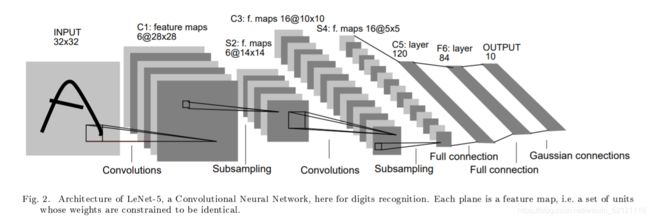
LeNet-5 网络结构
LeNet-5由七层组成（不包括输入层），每一层都包含可训练权重。

---

LeNet 代码实现

import torch
import torch.nn as nn
import torch.nn.functional as F
import matplotlib.pyplot as plt

class LeNet(nn.Module):
    def __init__(self):
        super().__init__()
        self.conv1 = nn.Conv2d(1, 20, kernal_size=(5, 5), stride=1)
        self.pool1 = nn.MaxPool2d(2)
        self.conv2 = nn.Conv2d(20, 50, kernel_size=(5, 5), stride=1)
        self.pool2 = nn.MaxPool2d(2)
        
        self.fc1 = nn.Linear(800, 500)
        self.relu1 = nn.ReLU()
        self.fc2 = nn.Linear()
        self.relu2 = nn.ReLU()
        
    def forward(self, x):
        x = self.pool1(self.conv1(x))
        x = self.pool2(self.conv2(x))
        x = self.relu1(self.fc1(x.view(-1, 800)))
        x = self.relu2(self.fc2(x))
        return F.log_softmax(x)
        

---

AlexNet

• 2012年，ImageNet 竞赛冠军获得者 Hinton 和其学生 Alex Krizhevsky 设计。
• 论文：ImageNet Classification with Deep Convolutional Neural Networks
  https://proceedings.neurips.cc/paper/2012/file/c399862d3b9d6b76c8436e924a68c45b-Paper.pdf

---

相比 LeNet 的优点：

• 网络结构更深，学习能力增强
  前五层都是卷积层，后三层为全连接层；使用 softmax 函数完成了 1000个类别的多分类任务；
• 使用了数据增强，增加了模型的泛化能力
  数据增强方式：随机裁剪、旋转角度、变换图片亮度等
• 引入了 DropOut，避免过拟合
  引入机器学习集成算法的思想，让FC的神经元以一定的概率失活（常用概率：50%），失活的神经元不参与前向传播和反向传播；经过 dropout 后，使用输出值除以失活概率以突出被选中的神经元。
• 引入局部响应归一化处理 LRN

---

其他特点

• 相比 LeNet 拥有更多卷积层，但结构和流程没有变化；受当时 GPU 设备限制，采用双 GPU 设备并行训练；
• LRN: Local Response Normalization，局部响应归一化

---

---

Dropout

a = torch.Tensor([[1, 2, 3, 4], [5, 6, 7, 8]])
b = nn.Dropout(0.5)
b(a)
'''
tensor([[ 0.,  0.,  0.,  8.],
        [10., 12., 14., 16.]])
'''

---

AlexNet 网络结构

---

torchvision中的AlexNet的实现

参考：https://blog.csdn.net/pengchengliu/article/details/108909195

import torch
import torch.nn as nn
from .utils import load_state_dict_from_url
 
 
__all__ = ['AlexNet', 'alexnet']
 
 
model_urls = {
    'alexnet': 'https://download.pytorch.org/models/alexnet-owt-4df8aa71.pth',
}
 
 
class AlexNet(nn.Module):
 
    def __init__(self, num_classes=1000):
        super(AlexNet, self).__init__()
        self.features = nn.Sequential(
            #conv1
            nn.Conv2d(3, 64, kernel_size=11, stride=4, padding=2),  # 3表示输入的图像是3通道的。64表示输出通道数，也就是卷积核的数量。
            nn.ReLU(inplace=True),
            nn.MaxPool2d(kernel_size=3, stride=2),
 
            #conv2
            nn.Conv2d(64, 192, kernel_size=5, padding=2),
            nn.ReLU(inplace=True),
            nn.MaxPool2d(kernel_size=3, stride=2),
 
            #conv3
            nn.Conv2d(192, 384, kernel_size=3, padding=1),
            nn.ReLU(inplace=True),
 
            #conv4
            nn.Conv2d(384, 256, kernel_size=3, padding=1),
            nn.ReLU(inplace=True),
 
            #conv5
            nn.Conv2d(256, 256, kernel_size=3, padding=1),
            nn.ReLU(inplace=True),
            nn.MaxPool2d(kernel_size=3, stride=2),
        )
        
        self.avgpool = nn.AdaptiveAvgPool2d((6, 6)) #如果输入的图片不是224*224，那上面的池化输出的就可能不是6*6。而下面的FC层要求的输入必须是6*6,否则就没法运算。
        self.classifier = nn.Sequential(
            #FC1
            nn.Dropout(),   #用于减轻过拟合
            nn.Linear(256 * 6 * 6, 4096),  #全连接层。输入的是前面的特征图。特征图是6*6大小的，有256个特征图。自己有4096个神经元。
            nn.ReLU(inplace=True),
 
            #FC2
            nn.Dropout(),
            nn.Linear(4096, 4096),
            nn.ReLU(inplace=True),
 
            #FC3
            nn.Linear(4096, num_classes), #num_classes:这里是1000.
        )
 
    def forward(self, x):
        x = self.features(x)
        x = self.avgpool(x)       #liupc:自适应的池化。
        x = torch.flatten(x, 1)   #拉成一个向量的形式。
        x = self.classifier(x)
        return x
 
 
def alexnet(pretrained=False, progress=True, **kwargs):
    r"""AlexNet model architecture from the `"One weird trick..." `_ paper.
    Args:
        pretrained (bool): If True, returns a model pre-trained on ImageNet 
        progress (bool): If True, displays a progress bar of the download to stderr
    """
    model = AlexNet(**kwargs)
    if pretrained:
        state_dict = load_state_dict_from_url(model_urls['alexnet'],
                                              progress=progress)
        model.load_state_dict(state_dict)
    return model 

---

ZFNet

论文：Visualizing and Understanding Convolutional Networks
https://arxiv.org/abs/1311.2901

---

• 是 2013年 ImageNet 竞赛中分类任务冠军
• 知名度不高。网络结构没有太大改进，只是在 AlexNet 基础上调节了参数，提升了分类性能。
• 在 AlexNet 基础上，ZFNet
  • 将第一个卷积层的卷积核由11变为7
  • stride 由4变为2
  • 后面卷积层依次变为 384、384、256
  • 增加了卷积层个数。

---

复现代码：

class ZFNer(nn.Module):
    def __init__(self):
        super().__init__()
        self.features = nn.Sequential(
            nn.Conv2d(3, 96, kernel_size=(7,7), stride=(2, 2)),
            nn.MaxPool2d((3, 3), stride=(2, 2)),
            nn.Conv2d(96, 256, kernel_size=(5,5), stride=(2, 2)),
            nn.MaxPool2d((3, 3), stride=(2, 2)),
            
            nn.Conv2d(256, 384, kernel_size=(3,3), stride=(1, 1)),
            nn.Conv2d(384, 384, kernel_size=(3,3), stride=(1, 1)),
            nn.Conv2d(384, 256, kernel_size=(3,3), stride=(1, 1)),
            
            nn.MaxPool2d((3, 3), stride=(2, 2)),
        )
        
        self.classifier = nn.Sequential(
            nn.Linear(43264, 4096),
            nn.ReLU(),
            nn.Dropout(),
            nn.Linear(4096, 4096),
            nn.ReLU(),
            nn.Dropout(),
            nn.Linear(4096, 1000)
        )
    
    def forward(self, x):
        
        x = self.features(x)
        x = x.view(-1, 43264)
        x = self.classifier(x)
        return x
        
    

---

VGG-Nets

• 2014年提出，牛津大学提出；获得定位任务第一名，分类任务第二名；
• VGG: Visual Geometry Group
• 使用了更深的网络结构，可看做 AlexNet 加深版；结构也沿用了 卷积层和全连接层。
  VGG-16、VGG-19 的明明说明了其网络结构层数（池化层不计算在内）；
• 为了解决权重初始化的问题，VGG 采用预训练的方式。

---

VGG 各网络

VGG 训练一小部分网络，在确保这部分网络稳定后，在此基础上加深。
下图提现的是这个过程，处于D阶段（VGG-16）的时候，效果最优。

---

VGG-16 网络结构

---

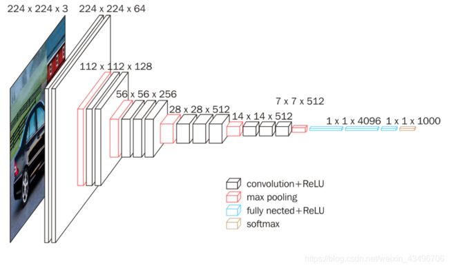
VGG-16 优点：结构更深，卷积层使用更小的卷积核尺寸和间隔。
小尺寸卷积核优点：

• 比大尺寸有更多的非线性，使判决函数更具有判决性；
• 有更少的参数。3个 3x3 卷积层参数个数为 3x3x3 = 27；一个 7x7 卷积层参数个数为 7x7 = 49。

---

GoogLeNet

• 2014年由Christian Szegedy提出。ImageNet 竞赛分类任务冠军。
• 在加深网络结构的同时，引入了 Inception 结构，代替卷积和激活函数。
  Inception 可参考文章： https://blog.csdn.net/weixin_43821559/article/details/123379833
  https://blog.csdn.net/weixin_44772440/article/details/122952961
• GoogLeNet 整个网络实际是 Inception 的堆叠。

---

• 论文：Going Deeper with Convolutions
  https://www.cv-foundation.org/openaccess/content_cvpr_2015/papers/Szegedy_Going_Deeper_With_2015_CVPR_paper.pdf

---

代码实现

class BasicConv2d(nn.Module):
    def __init__(self, in_channels, out_channels, **kwargs):
        super(BasicConv2d, self).__init__()
        self.conv = nn.Conv2d(in_channels, out_channels, bias=False, **kwargs)
        self.bn = nn.BatchNorm2d(out_channels, eps=0.01)
        
    def forward(self, x):
        x = self.conv(x)
        x = self.bn(x)
        return F.relu(x, inplace=True)
        
        
        
class Inception(nn.Module):
    def __init__(self, in_channels, pool_features):
        super(Inception, self).__init__()
        self.branch1X1 = BasicConv2d(in_channels, 64, kernel_size=1)
        self.branch5X5_1 = BasicConv2d(in_channels, 48, kernel_size=1)
        self.branch5X5_2 = BasicConv2d(48, 64, kernel_size=5, padding=2)
        
        self.branch3X3_1 = BasicConv2d(in_channels, 64, kernel_size=1)
        self.branch3X3_2 = BasicConv2d(64, 96, kernel_size=3, padding=1)
        self.branch_pool = BasicConv2d(in_channels, pool_features, kernel_size=1)
        
    def forward(self, x):
        branch1X1 = self.branch1X1(x)
        branch5X5 = self.branch5X5_1(x)
        branch5X5 = self.branch5X5_2(branch5X5)
        branch3X3 = self.branch3X3_1(x)
        branch3X3 = self.branch3X3_2(branch3X3)
        
        branch_pool = F.avg_pool2d(x, kernel_size=3, stride=1, padding=1)
        branch_pool = self.branch_pool(branch_pool)
        outputs = [branch1X1, branch3X3, branch5X5, branch_pool]
        
        return torch.cat(outputs, 1)
         

---

ResNet

• 2015年，何恺明推出；在 ISLVRC 和 COCO竞赛中获得冠军；
• 网络达到了152层，引入 残差单元 来解决梯度消失的问题；
  关于梯度消失：梯度是从后向前传播，增加梯度后，靠前的层梯度会很小（由链式法则造成）；这意味着这些曾基本上学习停滞，就是梯度消失问题。
  退化问题：网络更深，参数空间更大，优化问题更难。
• 论文: Deep Residual Learning for Image Recognition
  https://arxiv.org/abs/1512.03385

---

残差网络：
结构上看与电路的“短路”类似

---

代码实现

class Bottlenect(nn.Module):
    expansion = 4
    def __init__(self, inplanes, planes, stride=1, downsample=None):
        super(Bottlenect, self).__init__()
        self.conv1 = nn.Conv2d(inplanes, planes, kernel_size=1, bias=False)
        self.bn1 = nn.BatchNorm2d(planes)
        self.conv2 = nn.Conv2d(planes, planes, kernel_size=3, stride=stride, padding=1, bias=False)
        self.bn2 = nn.BatchNorm2d(planes)
        self.conv3 = nn.Conv2d(planes, planes * self.expansion, kernel_size=1, bias=False)
        self.bn3 = nn.BatchNorm2d(planes * self.expansion)
        self.relu = nn.ReLU(inplace=True)
        self.downsample = downsample
        self.stride = stride
    
    def forward(self, x):
        residual = x
        out = self.conv1(x)
        out = self.bn1(out)
        out = self.relu(out)
        out = self.conv2(out)
        out = self.bn2(out)
        out = self.relu(out)
        out = self.conv3(out)
        out = self.bn3(out)
        
        if self.downsample is not None:
            residual = self.downsample(x)
        
        out += residual
        out = self.relu(out)
        
        return out
    

---

DenseNet

• 获得 2017 CVPR 年度最佳论文
  Densely Connected Convolutional Networks
  https://arxiv.org/abs/1608.06993
• 思想上吸收了ResNet 和 Inception 结构的特点，设计了全新的网络结构。
• 是具有密集连接的CNN；任意两层之间都有直接的连接，就是说每层的输入都是前面所有层输入的并集；这种残差结构可以缓解梯度消失的现象。
• Dense 连接仅仅是在一个 DenseBlock 中，不同的 DenseBlock 之间是没有 Dense 连接的。
• DenseLayer 的 forward 方法中，最后的输出值是输入的x 和经过网络层输出的特征图cat 拼接在一起的。在 DenseBlock 中会遍历所有的layer，经过 DenseLayer 处理后，最终组合到 Sequentical 中，形成一个完整的 Block。
• 性能好，但是占用内存大；

---

网络结构

---

代码实现：

class _DenseLayer(nn.Sequential):
    def __init__(self, num_input_features, growth_rate, bn_size, drop_rate):
        super(_DenseLayer, self).__init__()
        self.add_module('norm1', nn.BatchNorm2d(num_input_features)), 
        self.add_module('relu1', nn.ReLU(inplace=True)),  
        self.add_module('conv1', nn.Conv2d(num_input_features, bn_size*growth_rate, kernel_size=1, stride=1, bias=False)),
        
        self.add_module('norm2', nn.BatchNorm2d(bn_size * growth_rate)),
        self.add_module('relu2', nn.ReLU(inplace=True)),
        self.add_module('conv2', nn.Conv2d(bn_size*growth_rate, growth_rate, kernel_size=3, stride=1, padding=1, bias=False)),
        
        self.drop_rate = drop_rate
        
    def forward(self, x):
        new_features = super(_DenseLayer, self).forward(x)
        if self.drop_rate > 0:
            new_features = F.dropout(new_features, p=self.drop_rate, training=self.training )
            
        return torch.cat([x, new_features], 1)
    
    
class _DenseBlock(nn.Sequential):
    
    def __init__(self, num_layers, num_input_features, bn_size, growth_rate, drop_rate):
        super(_DenseBlock, self).__init__()
        for i in range(num_layers):
            layer = _DenseLayer(num_input_features + i * growth_rate, growth_rate, bn_size, drop_rate)
            self.add_module('denselayer % d' % (i + 1), layer)
    
    

---

RNN

• 每个时刻的输入，都等于当前时刻的输入 和 上一时刻的记忆

• 论文: Recurrent Neural Networks as Weighted Language Recognizers
  https://arxiv.org/pdf/1711.05408.pdf

---

class RNNCell(nn.Module):
    def __init__(self, input_size, hidden_size, output_size, batch_size):
        super(RNNCell, self).__init__()
        self.batch_size = batch_size
        self.hidden_size = hidden_size
        self.i2h = nn.Linear(input_size + hidden_size, hidden_size)
        self.i2o = nn.Linear(input_size + hidden_size, output_size)
        self.softmax = nn.LogSoftmax(dim=1)
        
    def forward(self, input, hidden):
        combined = torch.cat((input, hidden), 1)
        hidden = self.i2h(combined)
        output = self.i2o(hidden)
        output = self.softmax(output)
        
    def initHidden(self):
        return torch.zeros(self.batch_size, self.hidden_size)
    
    
        

bias = 20 # 时间跨度
input_dim = 1 # 输入数据的维度
lr = 0.01 
epochs = 1000
hidden_size = 64 # 隐藏层神经元个数
num_layers = 2
nonlinearity = 'relu' # 只支持 relu 和 tanh

class RNNDemo(nn.Module):
    def __init__(self, input_dim, hidden_size, num_layers, nonlinearity):
        super().__init__()
        self.input_dim = input_dim
        self.hidden_size = hidden_size
        self.num_layers = num_layers
        self.nonlinearity = nonlinearity
        
        self.rnn = nn.RNN(
            input_size = input_dim,
            hidden_size = hidden_size,
            num_layers=num_layers,
            nonlinearity=nonlinearity
        )
        self.out = nn.Linear(hidden_size, 1)
        
    def forward(self, x, h):
        r_out, h_state = self.rnn(x, h)
        outs = []
        for record in range(r_out.size(1)):
            outs.append(self.out(r_out[:, record, :]))
        
        return torch.stack(outs, dim=1), h_state
        
        

# 使用 Adam 优化器，均方差误差训练模型

rnnDemo = RNNDemo(input_dim, hidden_size, num_layers, nonlinearity)
optimizer = torch.optim.Adam(rnnDemo.parameters(), lr=lr)
loss_func = nn.MSELoss()
h_state = None
for step in range(epoches):
    start, end = step * np.pi, (step + 1) * np.pi # 时间跨度
    
    # 使用三角函数 sin 预测 cos 的值
    steps = np.linspace(start, end, bins, dtype=np.float32, endpoint=False)
    x_np = np.sin(steps)
    y_np = np.cos(steps)
    
    # [100, 1, 1] 尺寸大小为 （time_step, batch, input_size）
    x = torch.from_numpy(x_np).unsqueeze(1).unsqueeze(2)
    y = torch.from_numpy(y_np).unsqueeze(1).unsqueeze(2) # [100, 1, 1]
    
    prediction, h_state = rnnDemo(x, h_state) # rnn输出（预测结果，隐藏状态）
    
    # 将每次输出的中间状态传递下去（不带梯度）
    h_state = h_state.detach()
    loss = loss_func(prediction, y)
    optimizer.zero_grad()
    loss.backward()
    optimizer.step()
    if (step%10) == 0:
        print('-- loss : {:.8f}'.format(loss) )
    
plt.scatter(steps, y_np, marker='^')
plt.scatter(steps, prediction.data.numpy().flatten(), marker='.')    
plt.show()

---

LSTM

• 1997 年提出
• 无力解决很长的上下文依赖。主要解决比较长的短时依赖，通常是10个间隔以内。
• 主要是三个门控单元：输入门、遗忘门（核心）、输出门。

---

代码实现

class LstmDemo(nn.Module):
    def __init__(self, input_dim, hidden_size, num_layers):
        super().__init__()
        self.input_dim = input_dim
        self.hidden_size = hidden_size
        self.num_layers = num_layers
        self.lstm = nn.LSTM(
            input_size = input_dim,
            hidden_size=hidden_size,
            num_layers=num_layers,
        )
        self.out = nn.Linear(hidden_size, 1)
        
    def forward(self, x, h_0_c_0):
        r_out, h_state = self.lstm(x, h_0,_c_0)
        outs = []
        # r_out:(h_n, c_n)
        for record in range(r_out.size(1)):
            outs.append(self.out(r_out[:, record, :]))
        
        return torch.stack(outs, dim=1), h_state
        
        

lstmDemo = LstmDemo(input_dim, hidden_size, num_layers).cuda()
optimizer = torch.optim.Adam(lstmDemo.parameters(), lr=lr)
loss_func = nn.MSELoss()

h_c_state = (torch.zeros(num_layers, 1, hidden_size).cuda(), torch.zeros(num_layers, 1, hidden_size).cuda() )

for step in range(epoches):
    start, end = step * np.pi, (step + 1) * np.pi # 时间跨度
    steps = np.linspace(start, end, bins, dtype=np.float32, endpoint=False)
    
    x_np = np.sin(steps)
    y_np = np.cos(steps)
    
    # [100, 1, 1] 尺寸大小为 （time_step, batch, input_size）
    x = torch.from_numpy(x_np).unsqueeze(1).unsqueeze(2).cuda()
    y = orch.from_numpy(y_np).unsqueeze(1).unsqueeze(2).cuda()
    
    prediction, h_state = lstmDemo(x, h_c_state)
    
    h_c_state = (h_state[0].detach(), h_state[1].detach() )
    loss = loss_func(prediction, y)
    optimizer.zero_grad()
    loss.backward()
    optimizer.step()
    if step % 100 == 0:
        print('-- loss : {:.8f}'.format(loss))
        
plt.scatter(steps, y_np, marker='^')
plt.scatter(steps, prediction.cpu().data.numpy().flatten(), marker='^')
plt.show()
     

---

GRU

• 与 LSTM 功能相同，简化了模型：将遗忘门和输入门合成一个单一的更新门；速度快于 LSTM。
• 论文: Empirical Evaluation of Gated Recurrent Neural Networks on Sequence Modeling
  https://arxiv.org/pdf/1412.3555.pdf

---

代码实现：

class GRUDemo(nn.Module):
    def __init__(self, input_dim, hidden_size, num_layers):
        super().__init__()
        self.input_dim = input_dim
        self.hidden_size = hidden_size
        self.num_layers = num_layers
        self.gru = nn.GRU(
            input_size = input_dim,
            hidden_size=hidden_size,
            num_layers=num_layers,
        )
        
        self.out = nn.Linear(hidden_size, 1)
        
    def forward(self, x, h):
        r_out, h_state = self.gru(x, h)
        outs = []
        for record in range(r_out.size[1]):
            outs.append(self.out(r_out[:, record, :]))
        return torch.stack(outs, dim=1), h_state
        

c_state = torch.zeros(num_layers, 1, hidden_size).cuda()

for step in range(epoches):
    start, end = step * np.pi, (step + 1) * np.pi # 时间跨度
    steps = np.linspace(start, end, bins, dtype=np.float32, endpoint=False)
    
    x_np = np.sin(steps)
    y_np = np.cos(steps)
    
    # [100, 1, 1] 尺寸大小为 （time_step, batch, input_size）
    x = torch.from_numpy(x_np).unsqueeze(1).unsqueeze(2).cuda()
    y = torch.from_numpy(y_np).unsqueeze(1).unsqueeze(2).cuda()
    
    prediction, c_state = gruDemo(x, c_state)
    
    c_state = c_state.detach() 
    loss = loss_func(prediction, y)
    optimizer.zero_grad()
    loss.backward()
    optimizer.step()
    
    if step % 100 == 0:
        print('-- loss : {:.8f}'.format(loss))
        
plt.scatter(steps, y_np, marker='^')
plt.scatter(steps, prediction.cpu().data.numpy().flatten(), marker='^')
plt.show()

---

2022-11-14（六）