均值漂移Mean Shift原理及推导过程

1.概述

Mean Shift的概念最早由Fukunage在1975年提出，后来由Yizong Cheng对其进行扩充，主要提出了两点的改进：一是定义了核函数，二增加了权重系数。核函数的定义使得偏移值对偏移向量的贡献随样本与被偏移点的距离的不同而不同，权重系数使得不同样本的权重有所不同。

均值漂移（mean-shift）算法是一种通用的寻找数据局部众数（local-mode）的搜索算法。它通常用于图像识别中的图像分割、目标跟踪、聚类和数据降维处理。

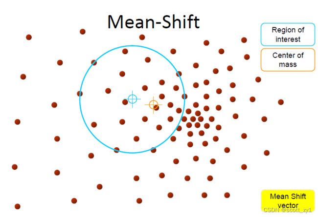
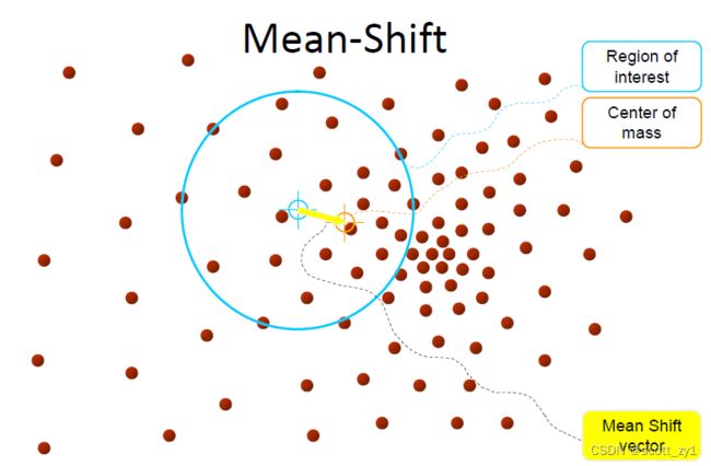
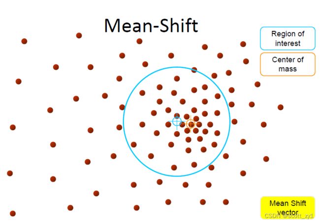
其实现思想如下：对于给定的一定数量样本，首先随便选择一个点作为中心点，然后计算该点一定范围之内所有点到中心点的距离向量的平均值作为偏移均值，然后将中心点移动到偏移均值位置(也就是该点范围内的质心)，通过这种不断重复的移动，可以使中心点逐步逼近到最佳位置。即选择的初始中心点会从沿一定变化方向移动到高密度中心点。具体实现过程示意图如下。

2.实现过程

2.1 核密度估计KDE

在讨论mean shift的具体实现过程之前，有必要先介绍核密度估计（KDE）。KDE是一种用来估计数据集潜在概率密度函数pdf的经典方法。它的工作原理是在数据集上的每一个样本点都设置一个核函数，然后对所有的核函数相加，得到数据集的核密度估计（kernel density estimation）。

为了具体的说明问题，假设我们有一个 维空间中点的数据 ，是从一些更大的总体数据集中采样得到的，并且我们选择了一个具有带宽参数 的kernel函数。那么基于总体的数据和核函数采用KDE方法就能实现对全部数据的概率密度估计，得到相应的pdf的一种近似。

                                                                                  (1)   

这里的核函数满足下面两个约束要求：

                                

                                                                   (2)   

-> 第一个要求是确保我们的估计是标准化（归一化）的。
-> 第二个与我们空间的对称性有关。

符号上述要求，比较常用的核函数由以下两个

                                            (3)              

                                        (4)   

如下图，采用高斯核估计一维数据集的密度，每个样本点都设置了以该样本点为中心的高斯分布，累加所有的高斯分布，得到该数据集的密度。

                

其中虚线表示每个样本点的高斯核，实线表示累加所有样本高斯核后的数据集密度。因此，我们通过高斯核来得到数据集的密度。

2.2 mean shift 推导

对于mean shift的推导过程，实现上述非参数估计pdf，定义径向对称核函数（如高斯核函数）​​​​​​​如下

                                                                                                (5)                        

那么定义某一数据样本,源于个独立同分布(i.i.d)的样本集，则对应的概率密度为，它的核密度估计如下：

        ​​​​​​​        ​​​​​​​                         (6)

 核密度函数的局部众数就是局部极大值，为了找到当前关注的样本点的核密度函数的局部极大值,对上式求偏导并令得到梯度表达式如式（7）：

​​​​​​​​​​​​​​

上式中最右边方括号内对应的一项就是所谓的均值漂移项（mean-shift），即:

        ​​​​​​​                ​​​​​​​                       (7)

取局部极大值时，对上述梯度设置为0，即对采用下述式迭代更新：

                                                                                (8)

上式就是均值漂移迭代更新，当迭代不再进行时即得到局部的众数.

由上式推导可知：均值漂移向量所指的方向是密度增加最大的方向。

算法的完整实现流程总结如下：

1.初始化随机种子位置并设定窗口大小对应的参数h。

2. 计算质心（平均值）。

3. 将搜索窗口移至质心位置，即叠加偏移量实现漂移。

4. 重复步骤 2 直至收敛

一般的算法流程（伪代码）

for p in copied_points:
    while not at_kde_peak:
        p = shift(p, original_points)

def shift(p, original_points):
    shift_x = float(0)
    shift_y = float(0)
    scale_factor = float(0)
  
    for p_temp in original_points:
        # numerator
        dist = euclidean_dist(p, p_temp)
        weight = kernel(dist, kernel_bandwidth)
        shift_x += p_temp[0] * weight
        shift_y += p_temp[1] * weight
        # denominator
        scale_factor += weight
  
    shift_x = shift_x / scale_factor
    shift_y = shift_y / scale_factor
    return [shift_x, shift_y]

动画演示效果如下：

3.算法总结

综合上述分析，总结mean shift作为实现数据聚类的方法，具有如下优点和不足

优点：

• 查找可变数量的众数（mode）
• 对异常值不敏感，有较好的鲁棒性
• 属于通用的、独立于应用程序的工具
• 无模型先验假设，在数据集群上不假设任何先前的形状，如球形、椭圆形等
• 只有一个参数（窗口大小 h），其中 h 具有物理意义（与 k-means 不同）

缺点：

• 聚类输出的质量取决于窗口大小的设定
• 窗口大小（带宽参数h）的设定非常关键，比较敏感
• 计算上（相对）耗时
• 不能很好地与特征空间的维度一起缩放

4.代码实现

4.1 python实现

import numpy as np
import math

MIN_DISTANCE = 0.00001  # 最小误差


def euclidean_dist(pointA, pointB):
    # 计算pointA和pointB之间的欧式距离
    total = (pointA - pointB) * (pointA - pointB).T
    return math.sqrt(total)


def gaussian_kernel(distance, bandwidth):
    ''' 高斯核函数
    :param distance: 欧氏距离计算函数
    :param bandwidth: 核函数的带宽
    :return: 高斯函数值
    '''
    m = np.shape(distance)[0]  # 样本个数
    right = np.mat(np.zeros((m, 1)))
    for i in range(m):
        right[i, 0] = (-0.5 * distance[i] * distance[i].T) / (bandwidth * bandwidth)
        right[i, 0] = np.exp(right[i, 0])
    left = 1 / (bandwidth * math.sqrt(2 * math.pi))
    gaussian_val = left * right
    return gaussian_val


def shift_point(point, points, kernel_bandwidth):
    '''计算均值漂移点
    :param point: 需要计算的点
    :param points: 所有的样本点
    :param kernel_bandwidth: 核函数的带宽
    :return:
        point_shifted：漂移后的点
    '''
    points = np.mat(points)
    m = np.shape(points)[0]  # 样本个数
    # 计算距离
    point_distances = np.mat(np.zeros((m, 1)))
    for i in range(m):
        point_distances[i, 0] = euclidean_dist(point, points[i])

    # 计算高斯核
    point_weights = gaussian_kernel(point_distances, kernel_bandwidth)

    # 计算分母
    all = 0.0
    for i in range(m):
        all += point_weights[i, 0]

    # 均值偏移
    point_shifted = point_weights.T * points / all
    return point_shifted


def group_points(mean_shift_points):
    '''计算所属的类别
    :param mean_shift_points:漂移向量
    :return: group_assignment：所属类别
    '''
    group_assignment = []
    m, n = np.shape(mean_shift_points)
    index = 0
    index_dict = {}
    for i in range(m):
        item = []
        for j in range(n):
            item.append(str(("%5.2f" % mean_shift_points[i, j])))

        item_1 = "_".join(item)
        if item_1 not in index_dict:
            index_dict[item_1] = index
            index += 1

    for i in range(m):
        item = []
        for j in range(n):
            item.append(str(("%5.2f" % mean_shift_points[i, j])))

        item_1 = "_".join(item)
        group_assignment.append(index_dict[item_1])
    return group_assignment


def train_mean_shift(points, kernel_bandwidth=2):
    '''训练Mean Shift模型
    :param points: 特征数据
    :param kernel_bandwidth: 核函数带宽
    :return:
        points：特征点
        mean_shift_points：均值漂移点
        group：类别
    '''
    mean_shift_points = np.mat(points)
    max_min_dist = 1
    iteration = 0
    m = np.shape(mean_shift_points)[0]  # 样本的个数
    need_shift = [True] * m  # 标记是否需要漂移

    # 计算均值漂移向量
    while max_min_dist > MIN_DISTANCE:
        max_min_dist = 0
        iteration += 1
        print("iteration : " + str(iteration))
        for i in range(0, m):
            # 判断每一个样本点是否需要计算偏置均值
            if not need_shift[i]:
                continue
            p_new = mean_shift_points[i]
            p_new_start = p_new
            p_new = shift_point(p_new, points, kernel_bandwidth)  # 对样本点进行偏移
            dist = euclidean_dist(p_new, p_new_start)  # 计算该点与漂移后的点之间的距离

            if dist > max_min_dist:  # 记录是有点的最大距离
                max_min_dist = dist
            if dist < MIN_DISTANCE:  # 不需要移动
                need_shift[i] = False

            mean_shift_points[i] = p_new
    # 计算最终的group
    group = group_points(mean_shift_points)  # 计算所属的类别
    return np.mat(points), mean_shift_points, group

4.2 调用sklearn

import numpy as np
from sklearn.cluster import MeanShift, estimate_bandwidth
data = []
f = open("k_means_sample_data.txt", 'r')
for line in f:
    data.append([float(line.split(',')[0]), float(line.split(',')[1])])
data = np.array(data)
# 通过下列代码可自动检测bandwidth值
# 从data中随机选取1000个样本，计算每一对样本的距离，然后选取这些距离的0.2分位数作为返回值，当n_samples很大时，这个函数的计算量是很大的。
bandwidth = estimate_bandwidth(data, quantile=0.2, n_samples=1000)
print(bandwidth)
# bin_seeding设置为True就不会把所有的点初始化为核心位置，从而加速算法
ms = MeanShift(bandwidth=bandwidth, bin_seeding=True)
ms.fit(data)
labels = ms.labels_
cluster_centers = ms.cluster_centers_
# 计算类别个数
labels_unique = np.unique(labels)
n_clusters = len(labels_unique)
print("number of estimated clusters : %d" % n_clusters)
# 画图
import matplotlib.pyplot as plt
from itertools import cycle
plt.figure(1)
plt.clf()  # 清楚上面的旧图形
# cycle把一个序列无限重复下去
colors = cycle('bgrcmyk')
for k, color in zip(range(n_clusters), colors):
    # current_member表示标签为k的记为true 反之false
    current_member = labels == k
    cluster_center = cluster_centers[k]
    # 画点
    plt.plot(data[current_member, 0], data[current_member, 1], color + '.')
    #画圈
    plt.plot(cluster_center[0], cluster_center[1], 'o',
             markerfacecolor=color,  #圈内颜色
             markeredgecolor='k',  #圈边颜色
             markersize=14)  #圈大小
plt.title('Estimated number of clusters: %d' % n_clusters)
plt.show()