基于R语言对股市价格预测的ARIMA建模
基于R语言对股市价格预测的ARIMA建模
获取数据
tushare ID=399224
利用ARIMA对股市价格进行拟合后预测,本次实验的数据源于tushare
首先导入本次实验所需要的所有包
require(zoo)     #na.trim
require(TTR)     #ROC
require(quantmod)
require(parallel)
require(xts)
require(Tushare)
require(fBasics)
require(tseries)
require(tsoutliers)
source("load_data.R")
本次实验以沪深300指数为例,下面读出从2015年1月1日至今的沪深300指数
df   <-get_data(data_function="index_daily",code="399300.SZ",start="20180101")
table<-to_zoo_format(df)
数据来自tushare平台
如果没有账号点击此处免费创建:https://tushare.pro/register?reg=399224
get_data函数来自于load_data.R文件:
require(zoo)    #na.trim
require(TTR)    #ROC
require(Tushare)
#///
#=================================#获取股票数据#================================
#///
get_data<-function(data_function='daily',code,start="",end="") {
    api <- Tushare::pro_api(token = 'YOUR TOKEN')#<<--输入你的TOKEN
    df  <- api(api_name = data_function, ts_code = code, start_date = start,end_date=end)
    df$trade_date <- as.character(df$trade_date)
    df$open <- as.character(df$open)
    df$high <- as.character(df$high)
    df$low <- as.character(df$low)
    df$close <- as.character(df$close)
    df$vol <- as.character(df$vol)

    df$open <- as.double(df$open)
    df$high <- as.double(df$high)
    df$low <- as.double(df$low)
    df$close <- as.double(df$close)
    df$vol <- as.double(df$vol)

    for (i in 1:length(df[,1]))
    {
        df[i,"trade_date"] <- paste(substr(df[i,"trade_date"], 1, 4),substr(df[i,"trade_date"], 5, 6),substr(df[i,"trade_date"], 7, 8),sep="-")
    }
    df
}

#///
#========================#读取tushare表格并转换#================================
#///
to_zoo_format <- function(company.raw)
{
  z <- zoo( cbind(	company.Open=company.raw$open,
                   company.High=company.raw$high,
                   company.Low=company.raw$low,
                   company.Close=company.raw$close,
                   company.Volume=company.raw$vol#,
                   #company.Adjusted=company.raw$Adj_C
  ),
  as.Date(company.raw$trade_date) )

  ret <- as.xts(z)

  ret
}
平稳性、白噪声的检验
平稳性的检验
方法1:可以根据时序图上看或者通过向光性的图中看出
先输出沪深300指数的K线图:
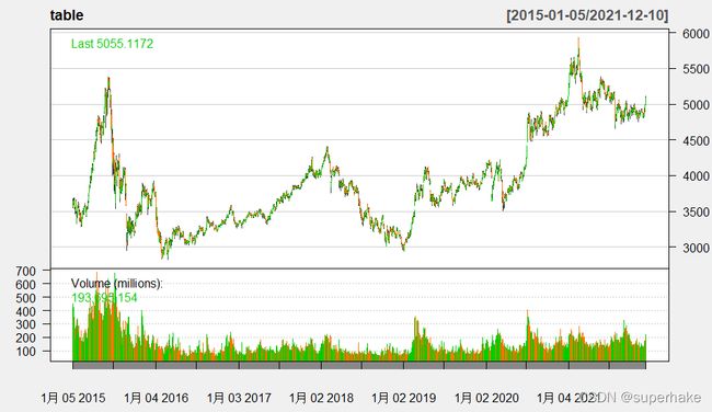
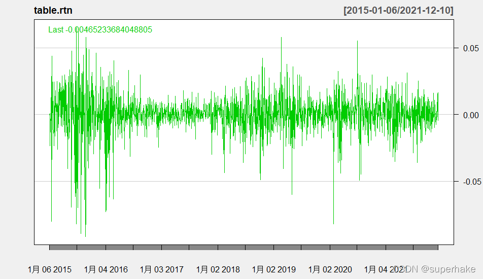
计算出对数收益率后输出时序图:
table.rtn <- diff(log(table$company.Close))

chartSeries(table.rtn,theme="white")
方法2:平稳序列通常具有短期相关性。该性质用自相关系数来描述就是随着延迟期数的增加,平稳序列的自相关系数会很快的衰减到0,特别,关于延迟的相关系数的计算公式如下
∑ i = 1 n − h ( x i − μ ^ ) ( x i + h − μ ^ 2 ) / ∑ i = 1 n ( x i − μ ^ ) 2 \sum_{i=1}^{n-h}({x_i}-\hat{\mu})({x_{i+h}-{\hat{\mu}}^2})/\sum_{i=1}^{n}(x_i-\hat{\mu})^2 i=1∑n−h(xi−μ^)(xi+h−μ^2)/i=1∑n(xi−μ^)2
其中
μ ^ = M e a n [ { x 1 , . . . , x n } ] \hat{\mu}=Mean[\{x_1,...,x_n\}] μ^=Mean[{x1,...,xn}]
在R语言当中可以使用tseries包的“adf.test”函数或者fUnitRoot包的adfTest函数
平稳性的检验方法还有DF-GLS检验、KPSS检验、PP检验与NP检验
ts <- na.omit(table.rtn)#由于差分后会产生空值,需要去除数据中的空值后进行adf检验
adf.test(ts, alternative = c("stationary", "explosive"))
Augmented Dickey-Fuller Test
data:  ts
Dickey-Fuller = -12.112, Lag order = 11, p-value = 0.01
alternative hypothesis: stationary
观察结果可知序列为平稳序列
判断是否是白噪音
白噪声没有研究的意义!
bartlett定理:
如果一个时间序列是纯随机的,得到一个观察期数为n的观察序列,那么该序列的延迟非零期的样本自相关系数将近似服从均值为零,方差为序列观察期数倒数的正态分布
ρ k ^ ∼ N ( 0 , 1 n ) , ∀ k ≠ 0 \hat{\rho_k}{\ }{\sim}{\ } N (0,\frac{1}{n}), \forall k\neq0 ρk^ ∼ N(0,n1),∀k=0
在R语言中可以使用Box.test函数来检验白噪音
# Ljung-Box统计量
##白噪音检验
for(i in 1:2) print(Box.test(ts,type = "Ljung-Box",lag=6*i))
#p<α 时拒绝零假设,α 为显著性水平。即认为序列不为白噪音
	Box-Ljung test

data:  ts
X-squared = 21.363, df = 6, p-value = 0.001579


	Box-Ljung test

data:  ts
X-squared = 36.163, df = 12, p-value = 0.000305
ARIMA模型建立
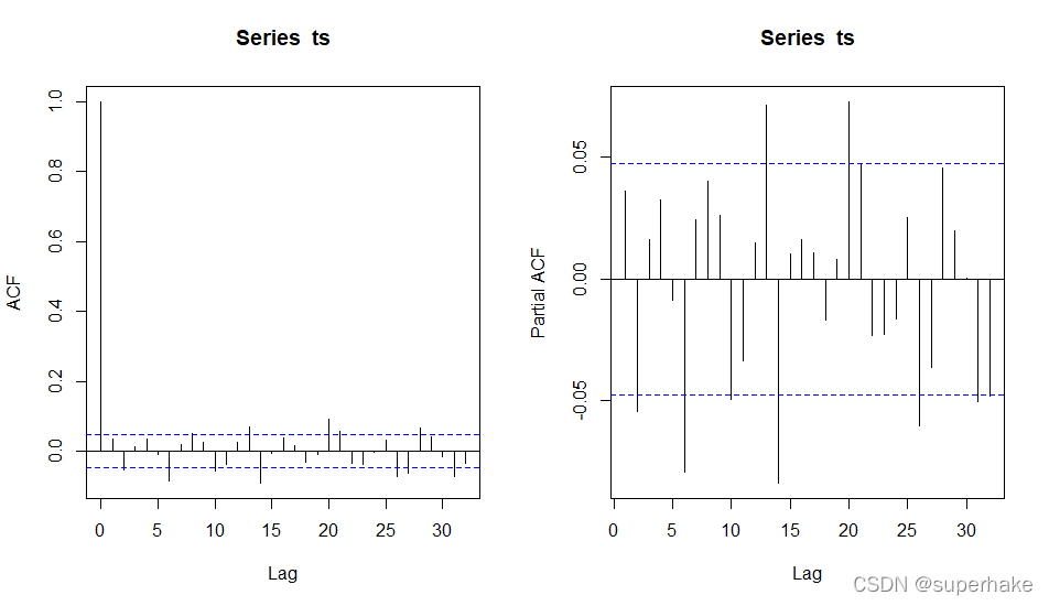
这里使用R里自带的auto.arima函数或者可以从ACF图与PACF图中确定p与q
绘制ACF与PACF图:
#部分自相关
par(mfrow = c(1,2))
acf(ts) # conventional ACF
pacf(ts) # pACF
model<-auto.arima(ts)
summary(model)
Series: ts
ARIMA(2,0,3) with zero mean

Coefficients:
         ar1      ar2      ma1     ma2     ma3
      0.1441  -0.9579  -0.1081  0.9186  0.0725
s.e.  0.0259   0.0146   0.0348  0.0220  0.0253

sigma^2 estimated as 0.0002171:  log likelihood=4729.3
AIC=-9446.61   AICc=-9446.56   BIC=-9414.01

Training set error measures:
                       ME       RMSE         MAE     MPE     MAPE     MASE         ACF1
Training set 0.0001872011 0.01471155 0.009980353 96.6115 201.7083 0.687844 0.0006095027
系统识别出的是ARIMA(2,0,3)模型,接下来我们使用系统识别出的模型来进行下面的步骤
对模型残差序列进行白噪音检验:
for(i in 1:2) print(Box.test(model$residual,lag=6*i))
	Box-Pierce test

data:  model$residual
X-squared = 2.8779, df = 6, p-value = 0.824


	Box-Pierce test

data:  model$residual
X-squared = 7.5982, df = 12, p-value = 0.8157
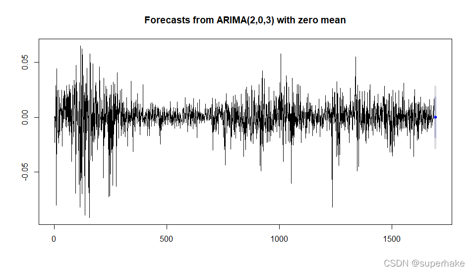
得到的结果为白噪音,下面对模型进行向后十步预测
library(forecast)
x.fore<-forecast(model,h=10)
x.fore
#系统默认输出预测图R
plot(x.fore)
     Point Forecast       Lo 80      Hi 80       Lo 95      Hi 95
1690  -0.0004786939 -0.01936027 0.01840288 -0.02935557 0.02839818
1691   0.0010980512 -0.01779570 0.01999181 -0.02779745 0.02999356
1692   0.0002677879 -0.01863697 0.01917254 -0.02864454 0.02918012
1693  -0.0010132974 -0.01992841 0.01790181 -0.02994146 0.02791487
1694  -0.0004024963 -0.01933085 0.01852585 -0.02935091 0.02854592
1695   0.0009127025 -0.01802218 0.01984759 -0.02804571 0.02987111
1696   0.0005170486 -0.01843268 0.01946677 -0.02846405 0.02949815
1697  -0.0007998362 -0.01975315 0.01815347 -0.02978642 0.02818675
1698  -0.0006105246 -0.01957952 0.01835847 -0.02962110 0.02840005
1699   0.0006782508 -0.01829229 0.01964879 -0.02833469 0.02969119