《Scikit Learn | MorvanZhou 》learning notes

学习资源

• https://scikit-learn.org/stable/
• https://morvanzhou.github.io/tutorials/machine-learning/sklearn/

---

1 Why Scikit Learn

Scikit learn 也简称 sklearn, 是机器学习领域当中最知名的 python 模块之一.

sklearn 包含

• Classification
• Regression
• Clustering
• Dimensionality reduction
• Model Selection
• Preprocessing

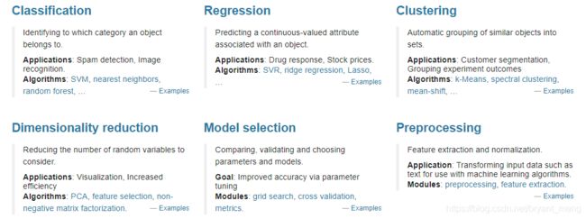
图片来源：https://scikit-learn.org/stable/

Sklearn 官网提供了一个速查手册（cheat-sheet），不同的判定条件、不同的任务场景采用对应的不同算法，大致是4类

• Classification
• Regression
• Clustering
• Dimensionality reduction

图片来源：https://scikit-learn.org/stable/tutorial/machine_learning_map/index.html

2 通用学习模式（牛刀小试 pipeline）

一招鲜吃遍天，了解一下，怎么使用 sklearn 来读数据，训练、测试模型！

我以 KNN 分类 iris 数据集为例，iris 数据集一共 150 个样本，输入 4 个特征，输出为 0/1/2 三类中的一种！我们把数据集按照 7：3 随机分成训练和测试集！

# View more python learning tutorial on my Youtube and Youku channel!!!

# Youtube video tutorial: https://www.youtube.com/channel/UCdyjiB5H8Pu7aDTNVXTTpcg
# Youku video tutorial: http://i.youku.com/pythontutorial

"""
Please note, this code is only for python 3+. If you are using python 2+, please modify the code accordingly.
"""
from __future__ import print_function
from sklearn import datasets
from sklearn.model_selection import train_test_split # 划分训练和测试数据集，shuffle
from sklearn.neighbors import KNeighborsClassifier # 导入模型

iris = datasets.load_iris()
iris_X = iris.data # 数据
iris_y = iris.target # 标签

print("feature shape：",iris_X.shape)
print("label shape：",iris_y.shape)
print("label:\n",iris_y)

X_train, X_test, y_train, y_test = train_test_split(
    iris_X, iris_y, test_size=0.3)

print("splited test label:\n", y_test)

knn = KNeighborsClassifier()
knn.fit(X_train, y_train)  # 开始训练

print("prediction:\n",knn.predict(X_test)) # 预测
print("ground truth:\n",y_test) # 对于测试集的 label

print("acc:",sum(knn.predict(X_test)==y_test)/len(y_test))

output

feature shape： (150, 4)
label shape： (150,)
label:
 [0 0 0 0 0 0 0 0 0 0 0 0 0 0 0 0 0 0 0 0 0 0 0 0 0 0 0 0 0 0 0 0 0 0 0 0 0
 0 0 0 0 0 0 0 0 0 0 0 0 0 1 1 1 1 1 1 1 1 1 1 1 1 1 1 1 1 1 1 1 1 1 1 1 1
 1 1 1 1 1 1 1 1 1 1 1 1 1 1 1 1 1 1 1 1 1 1 1 1 1 1 2 2 2 2 2 2 2 2 2 2 2
 2 2 2 2 2 2 2 2 2 2 2 2 2 2 2 2 2 2 2 2 2 2 2 2 2 2 2 2 2 2 2 2 2 2 2 2 2
 2 2]
splited test label:
 [0 1 1 0 1 2 2 1 2 0 2 1 0 0 0 2 2 0 2 1 2 2 1 0 1 1 1 2 2 0 0 0 2 0 2 2 1
 1 0 2 0 2 0 2 1]
prediction:
 [0 1 1 0 1 2 2 1 2 0 2 1 0 0 0 2 2 0 2 1 2 2 1 0 1 1 1 2 2 0 0 0 2 0 2 2 2
 2 0 2 0 2 0 2 1]
ground truth:
 [0 1 1 0 1 2 2 1 2 0 2 1 0 0 0 2 2 0 2 1 2 2 1 0 1 1 1 2 2 0 0 0 2 0 2 2 1
 1 0 2 0 2 0 2 1]
acc: 0.9555555555555556

可以看到 ACC还行，因为数据是 random shuffle 成 train 和 test data 的，所以，每一次运行结果不太一样，有的时候能到 100% 哟！

3 sklearn 强大数据库（Loaders / Sample Generator）

https://scikit-learn.org/stable/modules/classes.html#module-sklearn.datasets

可以导入现有的库，

例如 boston 数据集

samples 是 506，dimension 是 13，13 个 features

我们按照前面的流程走一遍，这里为了方便，就不再划分数据集了，整个数据集做为训练集

from __future__ import print_function
from sklearn import datasets
from sklearn.linear_model import LinearRegression
import matplotlib.pyplot as plt

loaded_data = datasets.load_boston()
data_X = loaded_data.data
data_y = loaded_data.target

print("feature shape：",data_X.shape)
print("label shape：",data_y.shape)
print("part of label：\n",data_y[:5]) # 看看部分标签

model = LinearRegression()
model.fit(data_X, data_y)

# 看前5个样本的预测值和标签
print(model.predict(data_X[:5, :])) 
print(data_y[:5])

output

feature shape： (506, 13)
label shape： (506,)
part of label：
 [24.  21.6 34.7 33.4 36.2]
[30.00821269 25.0298606  30.5702317  28.60814055 27.94288232]
[24.  21.6 34.7 33.4 36.2]

哈哈，不是很准，回归波动 10 以内，label 的范围是 -5~50

也可以自己生成数据集！

eg，生成线性回归数据集

from __future__ import print_function
from sklearn import datasets
import matplotlib.pyplot as plt

X, y = datasets.make_regression(n_samples=100, n_features=1, n_targets=1, noise=0)
plt.scatter(X, y)
plt.show()

X, y = datasets.make_regression(n_samples=100, n_features=1, n_targets=1, noise=10)
plt.scatter(X, y)
plt.show()

X, y = datasets.make_regression(n_samples=100, n_features=1, n_targets=1, noise=50)
plt.scatter(X, y)
plt.show()

噪声 noise 参数设置的越大，波动越明显

4 sklearn 常用属性与功能（model）

以 boston 数据集为例，samples 是 506，dimension 是 13，13 个 features

from sklearn import datasets
from sklearn.linear_model import LinearRegression

loaded_data = datasets.load_boston()
data_X = loaded_data.data
data_y = loaded_data.target

model = LinearRegression()
model.fit(data_X, data_y) # 整个数据集当成训练集

print(model.predict(data_X[:4, :])) # 预测前 4 个样本的结果

output

[30.00821269 25.0298606  30.5702317  28.60814055] 

1）斜率和截距

print(model.coef_) # 斜率。boston 的 dimension 是 13，所有 13 个对应的系数
print(model.intercept_) # 截距

$y=a_1{x}_1+a_2{x}_2+...+a_{13}{x}_{13}+b$

output

[-1.07170557e-01  4.63952195e-02  2.08602395e-02  2.68856140e+00
 -1.77957587e+01  3.80475246e+00  7.51061703e-04 -1.47575880e+00
  3.05655038e-01 -1.23293463e-02 -9.53463555e-01  9.39251272e-03
 -5.25466633e-01]
36.49110328036198

图片来自：https://scikit-learn.org/stable/modules/generated/sklearn.linear_model.LinearRegression.html#sklearn.linear_model.LinearRegression

2）查看模型已设置的参数，有些参数默认值不是 None

print(model.get_params())

output

{'copy_X': True, 'fit_intercept': True, 'n_jobs': 1, 'normalize': False}

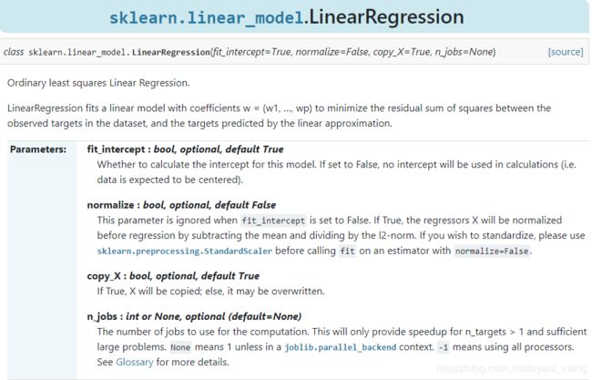
图片来自：https://scikit-learn.org/stable/modules/generated/sklearn.linear_model.LinearRegression.html#sklearn.linear_model.LinearRegression

3）给模型打分，LinearRegression 用的是 $R^2$

print(model.score(data_X, data_y)) # R^2 coefficient of determination

output

0.7406077428649428

$R^2$ 定义如下，参考 https://www.cnblogs.com/jiangkejie/p/10677858.html

5 正规化 Normalization

preprocessing.scale 是 Z-Score，也就减去均值除以标准差，处理后的数据具有 0 均值，单位标准差的特点！

from sklearn import preprocessing #标准化数据模块
import numpy as np

#建立Array
a = np.array([[10, 2.7, 3.6],
              [-100, 5, -2],
              [120, 20, 40]], dtype=np.float64)

# 计算每列的均值
a_mean = a.mean(axis=0)
print(a_mean,"\n")

# 计算每列的标准差
a_std = a.std(axis=0)
print(a_std,"\n")

# 标准化
b = (a-a_mean) / a_std
print(b,"\n")

c = preprocessing.scale(a)
print(c)

output

[10.          9.23333333 13.86666667] 

[89.8146239   7.67086841 18.61994152] 

[[ 0.         -0.85170713 -0.55138018]
 [-1.22474487 -0.55187146 -0.852133  ]
 [ 1.22474487  1.40357859  1.40351318]] 

[[ 0.         -0.85170713 -0.55138018]
 [-1.22474487 -0.55187146 -0.852133  ]
 [ 1.22474487  1.40357859  1.40351318]]

减均值除以方差后，数据预处理为零均值，单位方差的形式

print(c.mean(axis=0))
print(c.std(axis=0))

output

[0.00000000e+00 1.48029737e-16 0.00000000e+00]
[1. 1. 1.]

再比如把数据 0-1化

from sklearn import preprocessing #标准化数据模块
import numpy as np

#建立Array
a = np.array([[10, 2.7, 3.6],
              [-100, 5, -2],
              [120, 20, 40]], dtype=np.float64)

a_min = a.min(axis=0)
a_max = a.max(axis=0)

b = (a-a_min) / (a_max-a_min)
print(b,"\n")

c = preprocessing.minmax_scale(a,feature_range=(0,1))
print(c)

output

[[0.5        0.         0.13333333]
 [0.         0.13294798 0.        ]
 [1.         1.         1.        ]] 

[[0.5        0.         0.13333333]
 [0.         0.13294798 0.        ]
 [1.         1.         1.        ]]

下面看看数据标准化对模型结果的影响（以 Z-Score 为例）

# 标准化数据模块
from sklearn import preprocessing 
import numpy as np

# 将资料分割成train与test的模块
from sklearn.model_selection import train_test_split

# 生成适合做classification资料的模块
from sklearn.datasets.samples_generator import make_classification 

# Support Vector Machine中的Support Vector Classifier
from sklearn.svm import SVC 

# 可视化数据的模块
import matplotlib.pyplot as plt 

#生成具有2种属性的300笔数据
X, y = make_classification(
    n_samples=300, n_features=2,
    n_redundant=0, n_informative=2, 
    random_state=22, n_clusters_per_class=1, 
    scale=100)

#可视化数据
plt.scatter(X[:, 0], X[:, 1], c=y)
plt.show()

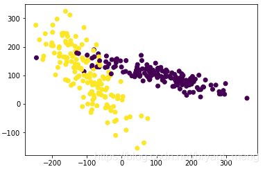
不 Z-Score 数据，用 SVM 分类试试，看下结果

X_train, X_test, y_train, y_test = train_test_split(X, y, test_size=0.3)
clf = SVC()
clf.fit(X_train, y_train)
print(clf.score(X_test, y_test))

0.45555555555555555

数据归一化处理后，再看看分类的结果

X = preprocessing.scale(X)
X_train, X_test, y_train, y_test = train_test_split(X, y, test_size=0.3)
clf = SVC()
clf.fit(X_train, y_train)
print(clf.score(X_test, y_test))

0.9666666666666667

提升到了 0.9 以上

6