pot lib：optimal transport python库

transport

https://github.com/rpetit/color-transfer
Rabin, J., & Papadakis, N. (2014). Non-convex relaxation of optimal transport for color transfer.

https://github.com/RachelBlin/Colorization-optimal-transport
Adaptive color transfer with relaxed optimal transport" by Rabin et. al.

A non parametric approach for histogram
segmentation 一种根据直方图分布的图像分割算法。

Optimal Transportation for Example-Guided Color Transfer 颜色转换

https://github.com/search?q=Optimal+Transport

1. 计算最优传输（Computational Optimal Transport）

介绍距离矩阵 和 概念

2. 离散测度 (Discrete measures), 蒙日(Monge)问题, Kantorovich Relaxation (松弛的蒙日问题)

最优运输（Optimal Transfort）：从理论到填补的应

3. scipy.stats.wasserstein_distance 距离计算

转化为累计直方图的差异。
還看不懂Wasserstein Distance嗎?看看這篇

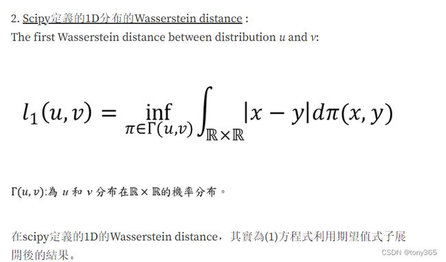
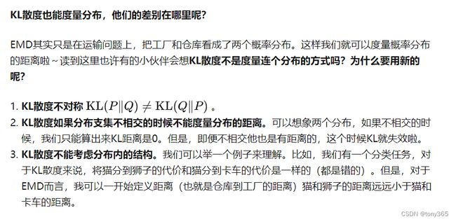
4. 转化为线性方程求解 Wasserstein距离 ， KL散度的对比分析

Wasserstein距离

5. pytorch 通过Sinkhorn 方法计算 Wasserstein距离

想要算一算Wasserstein距离？这里有一份PyTorch实战

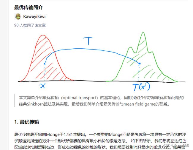
6. sinkhorn 原理：

最优传输简介

7. 解决方案

8. KL散度

https://zhuanlan.zhihu.com/p/527799934

9. book

Computational Optimal Transport
https://arxiv.org/pdf/1803.00567v4.pdf

pot lib

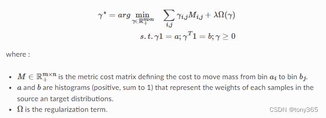
1 问题目标

将一个分布转移到另一个分布，做最小的功

主要应用：
1）测量两个分布的相似性，尤其是对于没有相同因变量（support）的分布
2）获得两个分布的mapping 关系。

1. Wasserstein distance between distributions

用于测量两个分布的距离或相似度。

2. mapping
   OT问题的一个非常有趣的方面是OT映射本身。当计算离散分布之间的最佳传输时，一个输出是OT矩阵，它将为您提供每个分布中样本之间的对应关系.

3. ot.optim.cg

   是一个通用的OT问题求解器，可以利用各种平滑连续约束。
   generic OT solver ot.optim.cg that can solve OT problems with any smooth/continuous regularization term making it particularly practical for research purpose.

4. 规模大的问题用 geomloss, 兼容pytorch

2 ot.emd 方法

[外链图片转存失败,源站可能有防盗链机制,建议将图片保存下来直接上传(img-oPVkY2KA-1681721618643)(2023-04-12-13-11-15.png)]

# a and b are 1D histograms (sum to 1 and positive)
# M is the ground cost matrix
T = ot.emd(a, b, M)  # exact linear program

exact linear program 求精确解，复杂度是 O^3

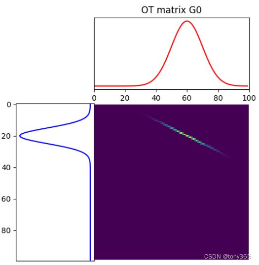
一维例子：
两个直方图以及他们的cost 矩阵

得到的结果

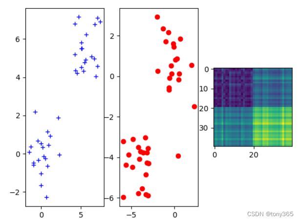
二维例子：
2D point, 每个点的概率相同（uniform）

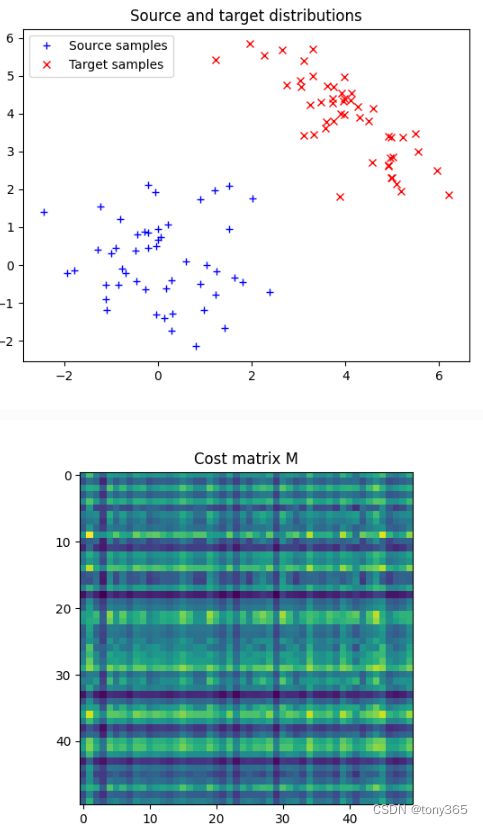
得到的结果和转换关系：

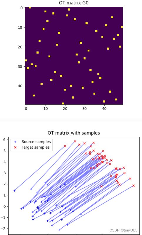
无论是一维还是二维，都是一些位置，另外就是把每个位置的值当作土堆的质量

3. ot.dist

采用不同的距离评价标准：

a, b = ot.unif(n), ot.unif(n)  # uniform distribution on samples

# loss matrix
M1 = ot.dist(xs, xt, metric='euclidean')
M1 /= M1.max()

# loss matrix
M2 = ot.dist(xs, xt, metric='sqeuclidean')
M2 /= M2.max()

# loss matrix
Mp = ot.dist(xs, xt, metric='cityblock')
Mp /= Mp.max()

得到不同的距离矩阵（cost matrix）：

最终得到的映射关系也是不同的：

4. 计算Wasserstein distance

可以通过计算出的转换矩阵T 与 cost matrix M对应相乘求和。
也可以通过 ot.emd2(a, b, M)

注意Wasserstein distance的公式：

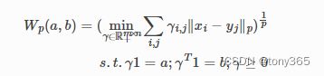
当p=1时， 利用 M = ot.dist(xs, xt, metric=‘euclidean’)
当p=2时， 利用 M = ot.dist(xs, xt) 默认是metric=‘seuclidean’, 因此调用ot.emd2后，还要求一个平方根，毕竟是 1/p

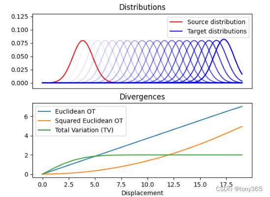
利用不同的M求解ot.emd2的效果：
分布距离越来越大，值也越来越大。

5. 特殊case:快速计算

再1D的情况下， ot.emd_1d, ot.emd2_1d, ot.wasserstein_1d 会有更好的计算效率。
另外就是如果两个分布都服从高斯分布，ot.gaussian.bures_wasserstein_mapping可以更快的计算。

6. Regularized Optimal Transport

正则化项1）提高计算效率，2）对于不同的应用可以设置不同的约束

具体来说有以下常见约束：

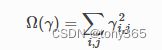
6.1 Entropic regularized OT

利用sinkhorn-knopp算法求解，函数是 ot.sinkhorn 和 ot.sinkhorn2.
lamda是一个超参数，控制 熵的大小，lamda越大，对转换矩阵的熵约束越弱，会使结果的熵更大，转换矩阵更加平滑。

The Sinkhorn-Knopp algorithm is implemented in ot.sinkhorn and ot.sinkhorn2 that return respectively the OT matrix and the value of the linear term.

主要函数是：（还有其他解法，没有一一列出。）

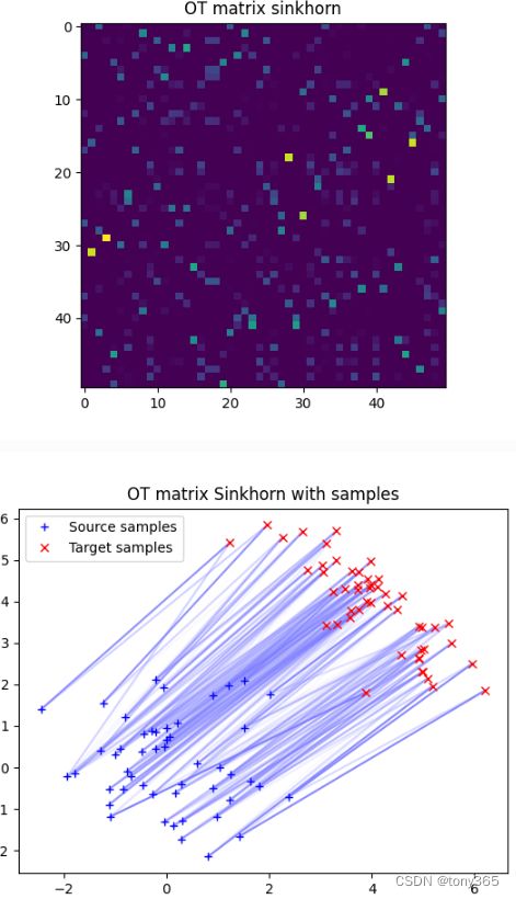
ot.sinkhorn
ot.sinkhorn2
ot.bregman.empirical_sinkhorn
ot.bregman.empirical_sinkhorn2

ot.sinkhorn实验：

# reg term
lambd = 1e-1

Gs = ot.sinkhorn(a, b, M, lambd)

ot.bregman.empirical_sinkhorn 实验：

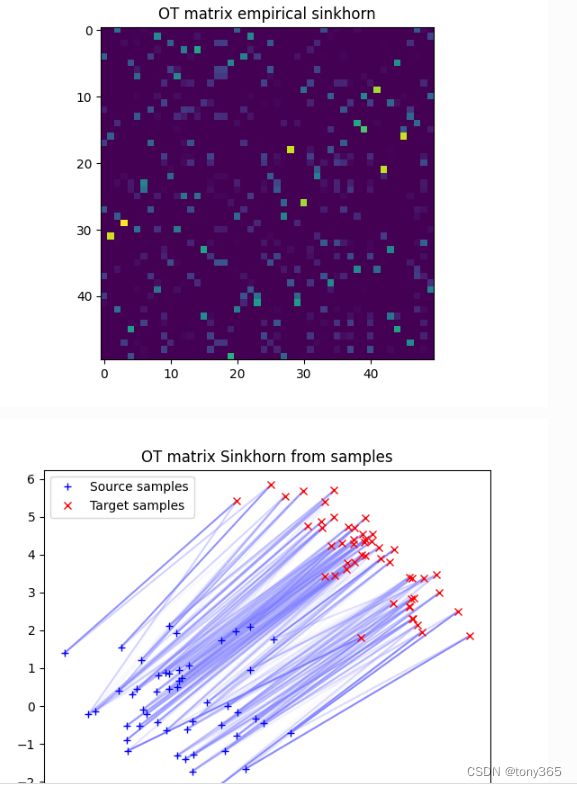
两者差不多。

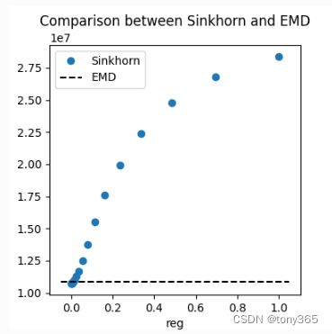
不同的lamda reg得到的 转换矩阵T不同：

损失也会随着lamda增大而变大。

6.2 Quadratic regularization 二次方约束

使用函数：

ot.smooth.smooth_ot_dual(a, b, M, lambd, reg_type='kl')
ot.smooth.smooth_ot_dual(a, b, M, lambd, reg_type='l2') # 这个是二次方约束
ot.smooth.smooth_ot_semi_dual

6.3 Group Lasso regularization

没有太理解其具体原理，它的作用是促进稀疏性，一般情况下 emd算法已经足够稀疏，所以这个约束并没有什么意义。 可以将它与 entropic regularization结合。

7 一个通用的约束框架

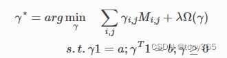
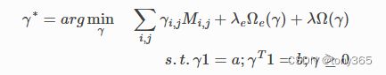
分别依赖ot.emd 和 ot.sinkhorn

函数分别是 ot.optim.cg 和 ot.optim.gcg
使用的时候需要定义正则化约束函数 和 其导数，通过这个方法可以实现各种正则化方法。

7.1 二范数正则化

def f(G):
    return 0.5 * np.sum(G**2)
def df(G):
    return G
reg = 1e-1
Gl2 = ot.optim.cg(a, b, M, reg, f, df, verbose=True)

7.2 entropic regularization

def f(G):
    return np.sum(G * np.log(G))
def df(G):
    return np.log(G) + 1.

reg = 1e-3
Ge = ot.optim.cg(a, b, M, reg, f, df, verbose=True)

7.3 平方 + entropic reg

def f(G):
    return 0.5 * np.sum(G**2)
def df(G):
    return G

reg1 = 1e-3
reg2 = 1e-1
Gel2 = ot.optim.gcg(a, b, M, reg1, reg2, f, df, verbose=True)

效果对比：

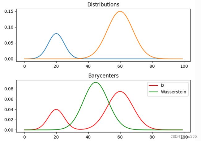
8. 求质心

alpha = 0.5  # 0<=alpha<=1
weights = np.array([1 - alpha, alpha])
# l2bary
bary_l2 = A.dot(weights)
# wasserstein
reg = 1e-3
ot.tic()
bary_wass = ot.bregman.barycenter(A, M, reg, weights)
ot.toc()
# linear exact
ot.tic()
bary_wass2 = ot.lp.barycenter(A, M, weights, solver='interior-point', verbose=True)
ot.toc()

以上三种方法的表现：

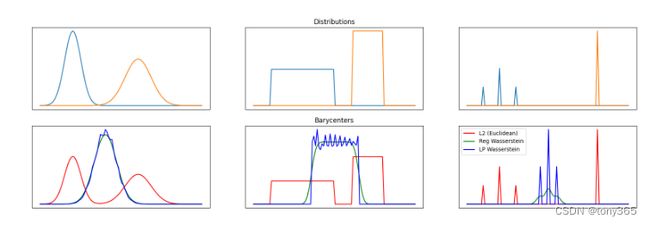
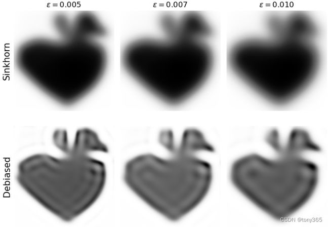
9. Debiased Sinkhorn barycenter 无偏质心

barycenter(A, M, reg, weights)
barycenter_debiased(A, M, reg, weights)
A是两个分布
效果对比如下：

对于2Dimage:
ot.bregman.convolutional_barycenter2d(A, reg, weights)
ot.bregman.convolutional_barycenter2d_debiased(A, reg, weights, log=True)
A 是多个图cancat在一起， reg是正则化系数，weights是 每个图的权重
最终效果如下：

10 unbalanced OT

数量不平衡，对转换矩阵的严格要求变为 正则化约束, 不要求完全a转到b， 因为两者的总数量也不同。

主要函数：

ot.sinkhorn_unbalanced
ot.sinkhorn_unbalanced2

entropic_kl_uot = ot.unbalanced.sinkhorn_unbalanced(a, b, M, reg, reg_m_kl)

# mm_unbalanced 不带 reg正则化项
kl_uot = ot.unbalanced.mm_unbalanced(a, b, M, reg_m_kl, div='kl')
l2_uot = ot.unbalanced.mm_unbalanced(a, b, M, reg_m_l2, div='l2')

质心：
bary_wass = ot.unbalanced.barycenter_unbalanced(A, M, reg, alpha, weights=weights)

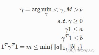
11. Partial optimal transport 部分转换

允许只tansport一部分：

w0, log0 = ot.partial.partial_wasserstein(p, q, M, m=0.5, log=True)
w, log = ot.partial.entropic_partial_wasserstein(p, q, M, reg=0.1, m=0.5,
                                                 log=True)
精确解 和 约束解

公式如下：

对于两个数据分布如下：

转换矩阵求得为：

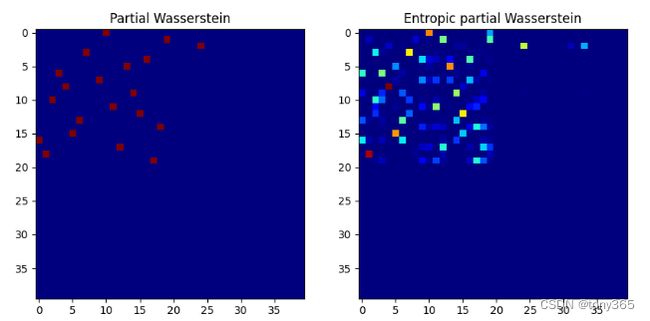
可以看出只进行了部分数据的转换。