Such complex, very wow – A guide to Algorithmic Complexity

Such complex, very wow – A guide to Algorithmic Complexity

Prerequisites:

• Exponentiation
• Basic algebra
• Functions and asymptotes
• Prior knowledge of Insertion Sort and other basic sorts of sorts

This post is roughly divided into three parts, so feel free to switch to either part depending on your level:

• Introduction
• Apprenticeship
• Mastery

---

Algorithmic complexity and growth of functions form the very foundation of algorithms. They give us an idea of how fast or slow an algorithm is, so you can’t go anywhere near designing and analyzing ’em without having these as tools.

Algosaurus wants to know what ‘growth of functions’ means. So he decides to get two bunnies. And the bunnies start having kids, hypothetically four per couple. Lots of them, because well, erm…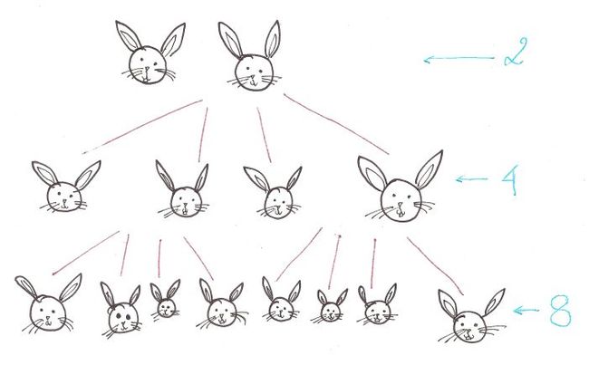

If we examine the growth of bunnies, we find that it grows at the rate of 2^n, where n is the number of generations. This isn’t very good news for Algosaurus, because despite bunnies being cute and cuddly, there issomething called having too many bunnies.

Roughly speaking, Bunny Breeding Algorithm has a complexity of O(2^n).

This is because the number of bunnies in next generation (the output) grows exponentially with respect to the number of bunnies we started with (the input).

Let’s dissect this.

“Order of growth of the running time of an algorithm gives a simple characterization of the algorithm’s efficiency and also allow us to compare the relative performance of alternative algorithms”.

– Holy Gospel of CLRS

Damn, that’s a mouthful.

Imagine Algosaurus is descending a very odd staircase with n stairs. To descend each stair, he has to walk ntiles horizontally, and only then he can step down.

So for each stair, he has to walk n tiles. Therefore, for n stairs, he must walk n^2 tiles.

def weirdStairs(nofStairs): steps = 0 for i in range(0, nofStairs): steps += nofStairs steps += 1 print steps

Total time taken to walk the entire flight of stairs?

---

Similarly, let’s take the example of the Insertion Sort.

def insertionSort(list): for i in range(1, len(list)): currentValue = list[i] position = index while position > 0 and list[position - 1] > currentValue: list[position] = list[position - 1] list[position] = currentValue 

Suppose the list is in descending order and every number has to be “inserted” into the right place, ie. each line of code in the loops is executed for every element.

As you go through the code, you’ll notice that for each element present in the list, it will have to iterate through the rest of elements in the list.

If n is the length of the list, the performance isn’t linearly proportional to n, it’s proportional to the square of n.

So, the worst case running time of the Insertion Sort comes out to be O(n^2), the ‘big-oh’ being part of standard notation and ‘n’ being the total number of elements in the list.

This is the worst case performance of the Insertion Sort, and usually the only kind of performance we care about.

We’ve only talked about lists with 10, maybe 100 elements. What about those with 1000, or even a million elements? Something like the total number of Facebook users?

Oh boy, then algorithmic complexity really begins to play a role.

The number of elements is so large in these cases, that only the highest power, ie. degree, of the polynomial matters, and nothing more. The rest of the terms are rendered insignificant.

The priority order for growth of functions is as follows: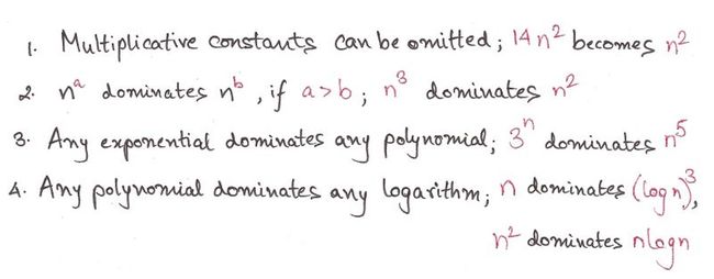
Also, roughly speaking, we can estimate the complexity of an algorithm by analyzing its loop structure.

Traversing a list is an O(n) operation, so is finding the length of one. This means running time is directly proportional to the number of elements.

def traversal(list): for i in range(len(list)): print list[i]

So at this point, Algosaurus knows enough about the growth of functions to figure out whether one algorithm is faster than the other. Yaaaaay.

For a more formal treatment of complexity analysis, read on. Or maybe come back to it after a cup of tea when all this has sunk in. *Subtle plug for bookmarking this page*

---

Opening CLRS page 43, Algosaurus sees…

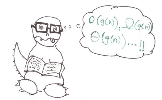Let’s first talk about ‘asymptotic notation’. As you probably know, when the input of certain functions tends to infinity, the output sometimes approaches a line, but doesn’t quite touch it. This line is called an asymptote.You should care because when designing a particular algorithm or implementing one, it is important to know how it will perform with huge input sizes. You already know what big-oh notation means: it tells you the worst-case performance of an algorithm. Let’s switch to big-omega. I’ll use the last example again. Suppose our input list is sorted to begin with, ie. the best-case performance.

def insertionSort(list): for i in range(1, len(list)): currentValue = list[i] position = index while position > 0 and list[position - 1] > currentValue: list[position] = list[position - 1] list[position] = currentValue 

We’ll still have to traverse every element in the list to determine whether it is sorted or not, even if we don’t go into the nested while loop. The outer loop is still executed ‘n’ times in the best case scenario.

So the best case performance turns out to Ω(n).

To digest what the rest of the godforsaken symbols mean, we need some math, namely…

Functions! And graphs!

Formally speaking, we can define Θ, O, and Ω as the following.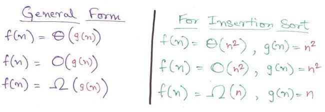

This doesn’t really mean much, to be honest. Let’s bring out the big guns: graphs. (Plugged from page 45 of CLRS)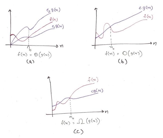

A few finer points. These functions are defined only when f(n) is monotonically adhering to the required constraints after n_0.

For example, for big-omega, Ω(g(n)) is formally defined only when it is less than the runtime of the function (c*g(n)) for all values greater than n_0.

a) This is for big-theta. It is sandwiched by two functions, showing that Θ(g(n)) is defined only when it is bound from the upper and the lower sides. You can’t just say it, you gotta prove it. Hard work.

b) This is for big-oh. The runtime function is always less than O(g(n)), showing that big-oh is the *upper bound* for the runtime. Actual performance won’t be worse than this.

c) For big-omega. The runtime function is always greater than Ω(g(n)), showing that big-omega is the *lower bound* for the runtime. You can’t do much better than this.

Patience Algosaurus. Here are the practical implications:

1. Big-omega is useful when you need a *lower bound* for the time, to show that an algorithm will always be slower than Ω(g(n)). Best-case performance.
Meh, sometimes used.

2. Big-oh is used when you need an *upper bound* for the time, to show that an algorithm will always be faster than O(g(n)). Worst-case performance.
Used all the time.

3. Finding big-theta is usually harder than big-oh, so big-oh is used more frequently, despite big-theta being more mathematically accurate. Math folks must find it blasphemous, but no can do.

Phew, that was a lot of theory.

---

I hope you found this informal guide to algorithmic complexity analysis useful. If you liked it, want to insult me, or if you want to talk about dinosaurs or whatever, shoot me a mail at [email protected]

Acknowledgements:
Introduction to Algorithms – Cormen, Leiserson, Rivest, and Stein (pages 43 – 64)
Algorithms – Dasgupta, Papadimitrou, and Vazirani (For the priority order)
Numbers: The Key to the Universe – Kjartan Poskitt (Bunny example inspired by this book)