深度学习笔记之Seq2Seq(一)基本介绍
深度学习笔记之Seq2seq——基本介绍
- 引言
-
- 回顾:经典循环神经网络结构
-
- 关于循环神经网络的更多引用
- Seq2seq \text{Seq2seq} Seq2seq网络结构
-
- Seq2seq \text{Seq2seq} Seq2seq结构描述
引言
从本节开始,将介绍 Seq2seq \text{Seq2seq} Seq2seq。
回顾:经典循环神经网络结构

在循环神经网络——循环神经网络思想中,我们介绍了经典循环神经网络结构。它的主要思想是:以序列信息作为媒介,给定序列数据 x ( 1 ) , x ( 2 ) , ⋯ , x ( T − 1 ) x^{(1)},x^{(2)},\cdots,x^{(\mathcal T-1)} x(1),x(2),⋯,x(T−1),求解下一时刻信息 x ( T ) x^{(\mathcal T)} x(T)的后验概率结果。
- 整个序列的联合概率分布 P ( X ) \mathcal P(\mathcal X) P(X)可表示为:
P ( x ( 1 ) , x ( 2 ) , ⋯ , x ( T ) ) = P ( x ( 1 ) ) ⋅ ∏ t = 2 T P ( x ( t ) ∣ x ( 1 ) , ⋯ , x ( t − 1 ) ) \mathcal P(x^{(1)},x^{(2)},\cdots,x^{(\mathcal T)}) = \mathcal P(x^{(1)}) \cdot \prod_{t=2}^{\mathcal T} \mathcal P(x^{(t)} \mid x^{(1)},\cdots,x^{(t-1)}) \\ P(x(1),x(2),⋯,x(T))=P(x(1))⋅t=2∏TP(x(t)∣x(1),⋯,x(t−1)) - 其中分解后的每一项(除去第一项),借助隐变量单元 h h h
{ P ( h ( t ) ∣ x ( t − 1 ) , h ( t − 1 ) ) P ( x ( t ) ∣ x ( t − 1 ) , h ( t ) ) t = 2 , 3 , ⋯ , T \begin{cases} \mathcal P(h^{(t)} \mid x^{(t-1)},h^{(t-1)}) \\ \mathcal P(x^{(t)} \mid x^{(t-1)},h^{(t)}) \end{cases} \quad t=2,3,\cdots,\mathcal T {P(h(t)∣x(t−1),h(t−1))P(x(t)∣x(t−1),h(t))t=2,3,⋯,T
对应地,它的前馈计算过程表示如下:
{ h ~ ( t + 1 ) = W h ( t ) ⇒ h ( t + 1 ) ⋅ h ( t ) + W x ( t ) ⇒ h ( t + 1 ) ⋅ x ( t ) + b h h ( t + 1 ) = σ ( h ~ ( t + 1 ) ) O ( t + 1 ) = ϕ ( W h ( t + 1 ) ⇒ O ( t + 1 ) ⋅ h ( t + 1 ) + b O ) \begin{cases} \begin{aligned} & \widetilde{h}^{(t+1)} = \mathcal W_{h^{(t)} \Rightarrow h^{(t+1)}} \cdot h^{(t)} + \mathcal W_{x^{(t)} \Rightarrow h^{(t+1)}} \cdot x^{(t)} + b_h \\ & h^{(t+1)} = \sigma(\widetilde{h}^{(t+1)}) \\ & \mathcal O^{(t+1)} = \phi(\mathcal W_{h^{(t+1)} \Rightarrow \mathcal O^{(t+1)}} \cdot h^{(t+1)} + b_{\mathcal O}) \end{aligned} \end{cases} ⎩ ⎨ ⎧h (t+1)=Wh(t)⇒h(t+1)⋅h(t)+Wx(t)⇒h(t+1)⋅x(t)+bhh(t+1)=σ(h (t+1))O(t+1)=ϕ(Wh(t+1)⇒O(t+1)⋅h(t+1)+bO)
这仅仅是 t ⇒ t + 1 t \Rightarrow t+1 t⇒t+1时刻的前馈计算过程,已知一段序列信息 X ∈ R n x × m × T \mathcal X \in \mathbb R^{n_x \times m \times \mathcal T} X∈Rnx×m×T:
这里使用的是 pytorch \text{pytorch} pytorch的向量格式。其中 n x n_x nx表示序列单元 x t ( t = 1 , 2 , ⋯ , T ) x_t(t=1,2,\cdots,\mathcal T) xt(t=1,2,⋯,T)的特征维数; m m m表示 BatchSize \text{BatchSize} BatchSize大小; T \mathcal T T表示序列单元的数量/序列长度。
X = [ x ( 1 ) , x ( 2 ) , ⋯ , x ( T ) ] T \mathcal X = [x^{(1)},x^{(2)},\cdots,x^{(\mathcal T)}]^T X=[x(1),x(2),⋯,x(T)]T
对应循环神经网络的输出 O \mathcal O O表示为:
这里的 n O n_{\mathcal O} nO表示经过神经元输出的特征维数。
O = [ O ( 1 ) , O ( 2 ) , ⋯ O ( T ) ] T ∈ R n O × m × T \mathcal O = [\mathcal O^{(1)},\mathcal O^{(2)},\cdots\mathcal O^{(\mathcal T)}]^T \in \mathbb R^{n_{\mathcal O} \times m \times \mathcal T} O=[O(1),O(2),⋯O(T)]T∈RnO×m×T
关于 LSTM,GRU \text{LSTM,GRU} LSTM,GRU网络结构同理,可以发现:输入与输出在序列维度上存在相同长度。
关于循环神经网络的更多引用
-
One to one \text{One to one} One to one模型结构。其网络结构表示如下:
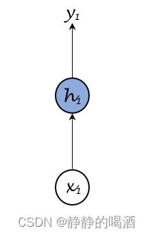
这里所说的 One to one \text{One to one} One to one是指序列信息并没有发生循环,相当于直接对输入数据进行分析并预测。可将视作一个全连接神经网络,相关任务如:图像分类。 -
One to many \text{One to many} One to many模型结构。其网络结构表示如下:
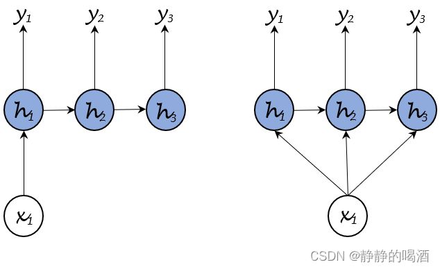
在隐藏状态发生循环的条件下,仅使用一个输入去预测一组序列输出。这类模型结构主要包含两种形式:- 唯一一个输入信息仅在初始时刻输入一次。代表任务如:文本生成;
- 唯一一个输入信息在每一时刻均输入一次。代表任务如:图像描述——将图像输入,并得到关于该图像的文字描述(文字序列)。
-
Many to one \text{Many to one} Many to one模型结构。其网络结构表示如下:
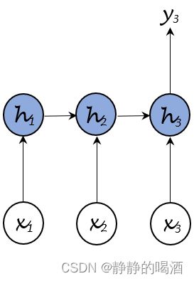
这种网络结构的特点在于:一个序列的输入得到最后时刻的输出,这使得该输出包含完整序列的特征信息。通过根据该信息执行判别任务。如:文本分类、情感分析等。 -
Many to many \text{Many to many} Many to many模型结构。其网络结构表示如下:

该网络结构的特点在于:基于一个序列的输入,生成另一个关联序列的输出。相关任务如:问答系统、机器翻译等。
其中输入序列和输出序列之间的关系不能狭隘地仅理解为语义相同,它也有可能存在‘语义之间存在因果关系’。像问答系统。
Seq2seq \text{Seq2seq} Seq2seq网络结构
从网络结构的角度观察, Seq2seq \text{Seq2seq} Seq2seq模型是由两个 RNN \text{RNN} RNN网络组成的网络结构。该模型广泛应用于自然语言处理的一些领域。如:机器翻译、文字识别等等。 Seq2seq \text{Seq2seq} Seq2seq的任务可理解为:从一个序列数据映射到另一个序列数据。相比于循环神经网络, Seq2seq \text{Seq2seq} Seq2seq的思想可表示为:
已知序列数据 X = ( x ( 1 ) , x ( 2 ) , ⋯ , x ( T ) ) \mathcal X = (x^{(1)},x^{(2)},\cdots,x^{(\mathcal T)}) X=(x(1),x(2),⋯,x(T))为条件,关于序列数据 Y = ( y ( 1 ) , y ( 2 ) , ⋯ , y ( T ′ ) ) \mathcal Y = (y^{(1)},y^{(2)},\cdots,y^{(\mathcal T')}) Y=(y(1),y(2),⋯,y(T′))的后验概率可表示为如下形式:
P ( y ( 1 ) , ⋯ , y ( T ′ ) ∣ x ( 1 ) , ⋯ , x ( T ) ) = P ( y ( 1 ) ∣ X ) ⋅ ∏ t = 2 T ′ P ( y ( t ) ∣ X , y ( 1 ) , ⋯ , y ( t − 1 ) ) \mathcal P(y^{(1)},\cdots,y^{(\mathcal T')} \mid x^{(1)},\cdots,x^{(\mathcal T)}) = \mathcal P(y^{(1)} \mid \mathcal X) \cdot \prod_{t=2}^{\mathcal T'} \mathcal P(y^{(t)} \mid \mathcal X,y^{(1)},\cdots,y^{(t-1)}) P(y(1),⋯,y(T′)∣x(1),⋯,x(T))=P(y(1)∣X)⋅t=2∏T′P(y(t)∣X,y(1),⋯,y(t−1))
上述公式可以看出, Seq2seq \text{Seq2seq} Seq2seq结构与循环神经网络的一个显著区别在于:关于输出序列 ( y ( 1 ) , y ( 2 ) , ⋯ , y ( T ′ ) ) (y^{(1)},y^{(2)},\cdots,y^{(\mathcal T')}) (y(1),y(2),⋯,y(T′))与输入序列,它们的序列长度可以不同。
Seq2seq \text{Seq2seq} Seq2seq结构描述
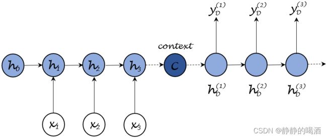
使用两个 RNN \text{RNN} RNN网络组成的 Seq2seq \text{Seq2seq} Seq2seq结构,一个被称作编码器 ( Encoder ) (\text{Encoder}) (Encoder),另一个被称作解码器 ( Decoder ) (\text{Decoder}) (Decoder)。
这里使用基于 PyTorch \text{PyTorch} PyTorch深度学习框架的代码进行描述。
- 关于编码器部分一般使用普通的 RNN \text{RNN} RNN系列结构,给定一组序列数据 { x ( 1 ) , x ( 2 ) , ⋯ , x ( T ) } \{x^{(1)},x^{(2)},\cdots,x^{(\mathcal T)}\} {x(1),x(2),⋯,x(T)},最终目标是将其表征为固定长度的 Context \text{Context} Context向量 C \mathcal C C:
这里的Context \text{Context} Context向量就是Encoder \text{Encoder} Encoder中RNN \text{RNN} RNN结构最终时刻的状态信息。它的大小与各时刻的隐藏状态大小相同。
该代码来自:序列到序列学习(Seq2seq)【动手学深度学习v2】
class Seq2SeqEncoder(nn.Module):

    def __init__(self,VocabSize,EmbedSize,NumHiddens,NumLayers,Dropout):
        super(Seq2SeqEncoder,self).__init__()

        self.VocabSize = VocabSize
        self.EmbedSize = EmbedSize
        self.Embedding = nn.Embedding(self.VocabSize,self.EmbedSize)
        self.RNN = nn.GRU(self.EmbedSize,NumHiddens,NumLayers,dropout=Dropout)

    def forward(self,x):
        x = self.Embedding(x)
        x = x.permute(1,0,2)
        Output,ContextState = self.RNN(x)
        return Output,ContextState
当然,上述的 Context \text{Context} Context向量仅是其中一种计算方式,这种计算方式并不唯一,根据不同情况的需要进行选择:
也可以对上述代码中的Output,ContextState \text{Output,ContextState} Output,ContextState构建一个单独的神经元,从而在中间过程增加一个关于Output,ContextState \text{Output,ContextState} Output,ContextState的复杂函数。并使用相应权重信息进行学习。其中h ( T ) h^{(\mathcal T)} h(T)表示Encoder \text{Encoder} Encoder结构中最后时刻T \mathcal T T生成的序列信息;函数f ( ⋅ ) f(\cdot) f(⋅)则表示由神经元构建的复杂函数。
{ C = h ( T ) C = f [ h ( T ) ] C = f [ h ( 1 ) , h ( 2 ) , ⋯ , h ( T ) ] \begin{cases} \begin{aligned} & \mathcal C = h^{(\mathcal T)} \\ & \mathcal C = f[h^{(\mathcal T)}] \\ & \mathcal C = f[h^{(1)},h^{(2)},\cdots,h^{(\mathcal T)}] \end{aligned} \end{cases} ⎩ ⎨ ⎧C=h(T)C=f[h(T)]C=f[h(1),h(2),⋯,h(T)]
关于解码器则负责基于 Context \text{Context} Context向量生成指定序列。它同样存在几种解码器结构。
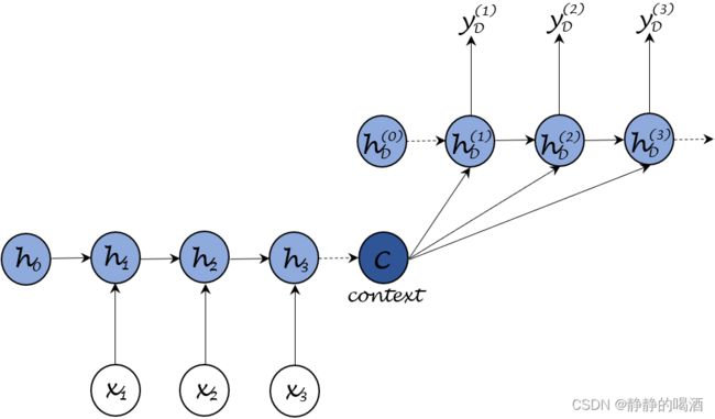
- 将编码器中产生的 Context \text{Context} Context向量——仅将其作为唯一的输入信息,并且该信息仅作用于初始时刻,并且不再添加其他额外信息。该解码器的网络结构表示如下:
该类型来源于博客Seq2Seq 模型详解,个人认为结构过于简单,甚至都不是循环神经网络的结构:
- 仅使用 Context \text{Context} Context信息作为输入,后续仅使用前一时刻的 Hidden State \text{Hidden State} Hidden State进行更新;
欢迎小伙伴们讨论。
它的隐藏状态更新过程以及各时刻输出表示如下:
其中符号 h D ( t ) ( t = 1 , 2 , ⋯ , T ′ ) h_{\mathcal D}^{(t)}(t=1,2,\cdots,\mathcal T') hD(t)(t=1,2,⋯,T′)表示 Decoder \text{Decoder} Decoder各时刻的隐藏层状态; y D ( t ) ( t = 1 , 2 , ⋯ , T ′ ) y_{\mathcal D}^{(t)}(t=1,2,\cdots,\mathcal T') yD(t)(t=1,2,⋯,T′)表示 Decoder \text{Decoder} Decoder各时刻的输出结果,下同。
Hidden state Update : { h D ( 1 ) = σ ( W C ⇒ h D ( 1 ) ⋅ C + b h D ) h D ( t ) = σ ( W h D ( t − 1 ) ⇒ h D ( t ) ⋅ h D ( t − 1 ) + b h D ) Output : y D ( t ) = σ ( W h D ( t ) ⇒ y D ( t ) ⋅ h D ( t ) + b y D ) \begin{aligned} & \text{Hidden state Update : }\begin{cases} h_{\mathcal D}^{(1)} = \sigma \left(\mathcal W_{\mathcal C \Rightarrow h_{\mathcal D}^{(1)}} \cdot \mathcal C + b_{h_{\mathcal D}} \right) \\ h_{\mathcal D}^{(t)} = \sigma \left(\mathcal W_{h_{\mathcal D}^{(t-1)} \Rightarrow h_{\mathcal D}^{(t)}} \cdot h_{\mathcal D}^{(t-1)} + b_{h_{\mathcal D}}\right) \end{cases} \\ & \text{Output : } y_{\mathcal D}^{(t)} = \sigma \left(\mathcal W_{h_{\mathcal D}^{(t)} \Rightarrow y_{\mathcal D}^{(t)}} \cdot h_{\mathcal D}^{(t)} + b_{y_{\mathcal D}}\right) \end{aligned} Hidden state Update : ⎩ ⎨ ⎧hD(1)=σ(WC⇒hD(1)⋅C+bhD)hD(t)=σ(WhD(t−1)⇒hD(t)⋅hD(t−1)+bhD)Output : yD(t)=σ(WhD(t)⇒yD(t)⋅hD(t)+byD)
- 和第一种情况相似—— Context \text{Context} Context向量依然作为唯一的输入信息,并且仅作用于初始时刻,区别在于将各时刻的输出结果作为下一时刻的输入信息。其解码器网络结果表示如下:
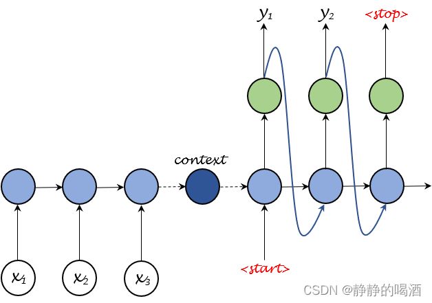
对应的隐藏状态更新过程以及各时刻输出表示如下:
Hidden state Update : { h D ( 1 ) = σ ( W C ⇒ h D ( 1 ) ⋅ C + W ⟨ start ⟩ ⇒ h D ( 1 ) ⋅ ⟨ start ⟩ + b h D ) h D ( t ) = σ ( W y D ( t − 1 ) ⇒ h D ( t ) ⋅ y D ( t − 1 ) + W h D ( t − 1 ) ⇒ h D ( t ) ⋅ h D ( t − 1 ) + b h D ) Output : y D ( t ) = σ ( W h D ( t ) ⇒ y D ( t ) ⋅ h D ( t ) + b y D ) \begin{aligned} & \text{Hidden state Update : }\begin{cases} h_{\mathcal D}^{(1)} = \sigma \left(\mathcal W_{\mathcal C \Rightarrow h_{\mathcal D}^{(1)}} \cdot \mathcal C + \mathcal W_{\left\langle\text{start}\right\rangle \Rightarrow h_{\mathcal D}^{(1)}} \cdot \left\langle \text{start}\right\rangle + b_{h_{\mathcal D}}\right) \\ h_{\mathcal D}^{(t)} = \sigma \left(\mathcal W_{y_{\mathcal D}^{(t-1)} \Rightarrow h_{\mathcal D}^{(t)}} \cdot y_{\mathcal D}^{(t-1)} + \mathcal W_{h_{\mathcal D}^{(t-1)} \Rightarrow h_{\mathcal D}^{(t)}} \cdot h_{\mathcal D}^{(t-1)} + b_{h_{\mathcal D}}\right) \end{cases} \\ & \text{Output : } y_{\mathcal D}^{(t)} = \sigma \left(\mathcal W_{h_{\mathcal D}^{(t)} \Rightarrow y_{\mathcal D}^{(t)}} \cdot h_{\mathcal D}^{(t)} + b_{y_{\mathcal D}}\right) \end{aligned} Hidden state Update : ⎩ ⎨ ⎧hD(1)=σ(WC⇒hD(1)⋅C+W⟨start⟩⇒hD(1)⋅⟨start⟩+bhD)hD(t)=σ(WyD(t−1)⇒hD(t)⋅yD(t−1)+WhD(t−1)⇒hD(t)⋅hD(t−1)+bhD)Output : yD(t)=σ(WhD(t)⇒yD(t)⋅hD(t)+byD) - 第三种解码器结构—— Context \text{Context} Context向量依然作为唯一的的输入信息,与之前不同的是,该向量作用于解码过程中的任意时刻。其解码器网络结构表示如下:
它可看作是‘第一种’的延伸。
对应的隐藏状态更新过程以及各时刻输出表示如下:
{ Hidden State Update : h D ( t ) = σ ( W C ⇒ h D ( t ) ⋅ C + W h D ( t − 1 ) ⇒ h D ( t ) ⋅ h D ( t − 1 ) + b h D ) Output : y D ( t ) = σ ( W h D ( t ) ⇒ y D ( t ) ⋅ h D ( t ) + b y D ) \begin{aligned} \begin{cases} &\text{Hidden State Update : } h_{\mathcal D}^{(t)} = \sigma \left(\mathcal W_{\mathcal C \Rightarrow h_{\mathcal D}^{(t)}} \cdot \mathcal C + \mathcal W_{h_{\mathcal D}^{(t-1)} \Rightarrow h_{\mathcal D}^{(t)}} \cdot h_{\mathcal D}^{(t-1)} + b_{h_{\mathcal D}}\right) \\ & \text{Output : } y_{\mathcal D}^{(t)} = \sigma \left(\mathcal W_{h_{\mathcal D}^{(t)} \Rightarrow y_{\mathcal D}^{(t)}} \cdot h_{\mathcal D}^{(t)} + b_{y_{\mathcal D}}\right) \end{cases} \end{aligned} ⎩ ⎨ ⎧Hidden State Update : hD(t)=σ(WC⇒hD(t)⋅C+WhD(t−1)⇒hD(t)⋅hD(t−1)+bhD)Output : yD(t)=σ(WhD(t)⇒yD(t)⋅hD(t)+byD)
- 第四种解码器结构——在第三种的基础上,将各时刻的输出信息作为下一时刻的输入信息。其解码器网络结构表示如下:
第二种与第三种的结合版。
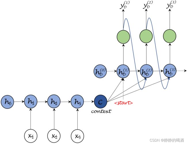
对应的隐藏状态更新过程以及各时刻输出表示如下:
{ Hidden State Update : h D ( t ) = σ ( W C ⇒ h D ( t ) ⋅ C + W h D ( t − 1 ) ⇒ h D ( t ) ⋅ h D ( t − 1 ) + W y D ( t − 1 ) ⇒ h D ( t ) ⋅ y D ( t − 1 ) + b h D ) Output : y D ( t ) = σ ( W h D ( t ) ⇒ y D ( t ) ⋅ h D ( t ) + b y D ) \begin{aligned} \begin{cases} &\text{Hidden State Update : } h_{\mathcal D}^{(t)} = \sigma \left(\mathcal W_{\mathcal C \Rightarrow h_{\mathcal D}^{(t)}} \cdot \mathcal C + \mathcal W_{h_{\mathcal D}^{(t-1)} \Rightarrow h_{\mathcal D}^{(t)}} \cdot h_{\mathcal D}^{(t-1)} + \mathcal W_{y_{\mathcal D}^{(t-1)} \Rightarrow h_{\mathcal D}^{(t)}} \cdot y_{\mathcal D}^{(t-1)} + b_{h_{\mathcal D}}\right) \\ & \text{Output : } y_{\mathcal D}^{(t)} = \sigma \left(\mathcal W_{h_{\mathcal D}^{(t)} \Rightarrow y_{\mathcal D}^{(t)}} \cdot h_{\mathcal D}^{(t)} + b_{y_{\mathcal D}}\right) \end{cases} \end{aligned} ⎩ ⎨ ⎧Hidden State Update : hD(t)=σ(WC⇒hD(t)⋅C+WhD(t−1)⇒hD(t)⋅hD(t−1)+WyD(t−1)⇒hD(t)⋅yD(t−1)+bhD)Output : yD(t)=σ(WhD(t)⇒yD(t)⋅hD(t)+byD) - 还有一种解码器结构,来自于序列到序列学习(Seq2seq)【动手学深度学习v2】中沐神的代码解读。其思路是:将 Context \text{Context} Context向量复制成与解码器序列长度相同的数量,并将 Encoder \text{Encoder} Encoder的输入依次与 Context \text{Context} Context向量做拼接 (Concatenate) \text{(Concatenate)} (Concatenate),并将拼接结果作为输入的一部分,另一部分依然是 Context \text{Context} Context自身。对应解码器网络结构表示如下:

对应代码表示如下:
class Seq2SeqDecoder(nn.Module):
    def __init__(self,VocabSize,EmbedSize,Numhiddens,NumLayer,Dropout):
        super(Seq2SeqDecoder,self).__init__()

        self.VocabSize = VocabSize
        self.EmbedSize = EmbedSize
        self.Numhiddens = Numhiddens
        self.Numlayer = NumLayer

        self.Embedding = nn.Embedding(self.VocabSize,self.EmbedSize)
        self.RNN = nn.GRU(self.EmbedSize + self.Numhiddens,
                          self.Numhiddens,
                          self.Numlayer,
                          dropout=Dropout)
        self.Dense = nn.Linear(self.Numhiddens,self.VocabSize)

    def InitState(self,EncoderOutput):
        return EncoderOutput[1]

    def forward(self,x,State):
        x = self.Embedding(x)
        x = x.permute(1,0,2)

        Context = State[-1].repeat(x.shape[0],1,1)
        CatxContext = torch.cat((x,Context),2)
        Output,State = self.RNN(CatxContext,State)
        Output = self.Dense(Output).permute(1,0,2)
        return Output,State
即便它的模型结构变化较大,但是它依然没有跳出其核心思想:
P ( y ( 1 ) , ⋯ , y ( T ′ ) ∣ x ( 1 ) , ⋯ , x ( T ) ) = P ( y ( 1 ) ∣ X ) ⋅ ∏ t = 2 T ′ P ( y ( t ) ∣ X , y ( 1 ) , ⋯ , y ( t − 1 ) ) \mathcal P(y^{(1)},\cdots,y^{(\mathcal T')} \mid x^{(1)},\cdots,x^{(\mathcal T)}) = \mathcal P(y^{(1)} \mid \mathcal X) \cdot \prod_{t=2}^{\mathcal T'} \mathcal P(y^{(t)} \mid \mathcal X,y^{(1)},\cdots,y^{(t-1)}) P(y(1),⋯,y(T′)∣x(1),⋯,x(T))=P(y(1)∣X)⋅t=2∏T′P(y(t)∣X,y(1),⋯,y(t−1))
相关参考:
Seq2Seq 模型详解
序列到序列学习(Seq2seq)【动手学深度学习v2】
【神经网络】学习笔记十四——Seq2Seq模型