【图像处理】植物叶识别和分类

一、说明

        这是国外某个学生团队尝试用机器学习方法对植物叶进行识别分类的实验。实验给出若干张植物叶图片，针对这些图片，对特征进行测量、提取、重组，最后用机器学习方法实现；该具备一定的参考价值。

        现在是我们将图像处理学习应用于实际机器学习问题的时候了。对于这个博客，让我们解决一个涉及叶子的简单分类问题。作为小组作业，我们的团队得到了一个目录，其中包含来自各种植物的叶子图像。这些图像如下所示：

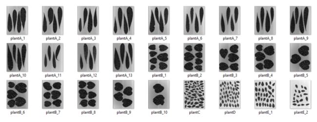
可以看出，在目录中可以找到 5 类叶子。因此，我们留下了这个机器学习问题：

我们可以使用传统的监督机器学习方法区分各种类别的叶子吗？
阅读直到本文末尾以找出答案。

二、特征提取

2.1 图像处理

        您可能会问的第一个问题，我们将在分析中使用哪些功能？为了使机器学习发挥作用，我们需要检查每个叶子类别共有的特征，以便算法可以决定叶子与其他叶子的区别。深度学习的进步，特别是卷积神经网络（CNN），使我们能够提取大量特征，并在大多数时间获得高精度分数。但是，由于这是一个关于使用图像处理技术的博客，我们不使用CNN。

        那么，如果我们不允许使用CNN从树叶中提取特征，那么首先将如何获得它们呢？这就是本博客的重点，使用图像处理来提取叶子特征，以便在Python中进行机器学习。

        与往常一样，必须导入以下库才能开始讨论：

from skimage.io import imshow, imread
 from skimage.color import rgb2gray
 from skimage.filters import threshold_otsu
 from skimage.morphology import closing
 from skimage.measure import label, regionprops, regionprops_table from sklearn.ensemble import GradientBoostingClassifier,      
    RandomForestClassifier
 from sklearn.model_selection import train_test_split
 from sklearn.metrics import classification_report from matplotlib import pyplot as plt
 import pandas as pd
 import numpy as np
 from tqdm import tqdm
 import os

        让我们看一下我们的一张灰度图像。运行下面的代码：​

 # get the filenames of the leaves under the directory “Leaves”
 image_path_list = os.listdir("Leaves") # looking at the first image
 i = 0
 image_path = image_path_list[i]
 image = rgb2gray(imread("Leaves/"+image_path))
 imshow(image)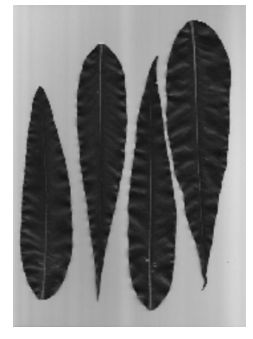

1）叶灰度图像

        现在，让我们开始使用 skimage '区域属性' 提取特征。但在此之前，我们需要预处理我们的图像，我们首先使用 Otsu 的方法对图像进行二值化，然后使用闭合形态操作对其进行清理。实现如下所示：

 binary = image < threshold_otsu(image)
 binary = closing(binary)
 imshow(binary)

2）叶子二值化图像：

                然后，我们可以标记预处理的图像以准备特征提取。

 label_img = label(binary)
 imshow(label_img)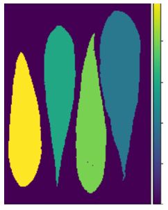

3）带标签的叶子图像

        最后，让我们使用区域属性从图像中提取特征。这种图像中，我们可以轻易地从每个图读出区域，测量区域的几何特征值。

2.2 特征测量值获取

        为了便于说明，让我们首先考虑这张图片。稍后我们将从每个叶子中提取特征。代码实现如下所示：

table = pd.DataFrame(regionprops_table(label_img, image,
                                       ['convex_area', 'area',
                                        'eccentricity', 'extent',                   
                                        'inertia_tensor',
                                        'major_axis_length', 
                                        'minor_axis_length'])) table['convex_ratio'] = table['area']/table['convex_area']
 table['label'] = image_path[5]
 table

        这将为我们提供一个数据帧，其中包含我们从函数调用regionprops_table功能。

        确实有可能获得特征。但是，这仅适用于一个图像。让我们获得其余部分的功能。怎么做？不用担心，这个博客可以满足您的需求。下面提供了有关如何执行此操作的代码实现：

image_path_list = os.listdir("Leaves")
df = pd.DataFrame()for i in range(len(image_path_list)):
   
  image_path = image_path_list[i]
  image = rgb2gray(imread("Leaves/"+image_path))
  binary = image < threshold_otsu(image)
  binary = closing(binary)
  label_img = label(binary)
  
  table = pd.DataFrame(regionprops_table(label_img, image
                          ['convex_area', 'area', 'eccentricity',
                           'extent', 'inertia_tensor',                         
                           'major_axis_length', 'minor_axis_length',
                           'perimeter', 'solidity', 'image',
                           'orientation', 'moments_central',
                           'moments_hu', 'euler_number',
                           'equivalent_diameter',
                           'mean_intensity', 'bbox']))  table['perimeter_area_ratio'] = table['perimeter']/table['area']  real_images = []
  std = []
  mean = []
  percent25 = []
  percent75 = []  for prop in regionprops(label_img): 
      
      min_row, min_col, max_row, max_col = prop.bbox
      img = image[min_row:max_row,min_col:max_col]
      real_images += [img]
      mean += [np.mean(img)]
      std += [np.std(img)]
      percent25 += [np.percentile(img, 25)] 
      percent75 += [np.percentile(img, 75)]  table['real_images'] = real_images
  table['mean_intensity'] = mean
  table['std_intensity'] = std
  table['25th Percentile'] = mean
  table['75th Percentile'] = std
  table['iqr'] = table['75th Percentile'] - table['25th Percentile']  table['label'] = image_path[5]
  df = pd.concat([df, table], axis=0)df.head()

2.3 从测量值到特征

        实现代码后，它为图像中的所有叶子生成了总共 51 个特征。现在，我们已经为机器学习的实施做好了准备。但在此之前，让我们解释一些提取以提供上下文的特征。

        我们根据区域属性计算了 4 个特征。

1. inertia_tensor — 这是一个表示惯性张量的元组。这与该段围绕其质量的旋转有关。注意，转动惯量是个有效物理指标，需要重视。

2. minor_axis_length — 这是指短轴的长度或段的较短轴。

3. solidity — 这只是凸包面积与二值图像面积的比率。

4. eccentricity — 偏心率是焦距（焦点之间的距离）与长轴长度的比值。

        我们还从灰度原始图像段中得出了这些属性。下面的所有功能都只是灰度值的统计信息。IQR 只是第 25 个百分位数和第 75 个百分位数的差值。

• 25th Percentile
• 75th Percentile
• mean_intensity
• std_intensity
• IQR

三、机器学习实现

        让我们继续机器学习实现。

X = df.drop(columns=['label', 'image', 'real_images'])#features
X = X[['iqr','75th Percentile','inertia_tensor-1-1',
       'std_intensity','mean_intensity','25th Percentile',
       'minor_axis_length', 'solidity', 'eccentricity']]#target
y = df['label']
columns = X.columns#train-test-split
X_train, X_test, y_train, y_test = train_test_split(
X, y, test_size=0.25, random_state=123, stratify=y)

        选择分类器算法。实验表明，表现最好的是梯度提升分类器。实现如下：

clf = GradientBoostingClassifier(n_estimators=50, max_depth=3, random_state=123)clf.fit(X_train, y_train)#print confusion matrix of test set
print(classification_report(clf.predict(X_test), y_test))#print accuracy score of the test set
print(f"Test Accuracy: {np.mean(clf.predict(X_test) ==            
                             y_test)*100:.2f}%")

        运行上述算法可提供以下结果：

四、分类报告

        性能最好的算法是GBM，因为它的测试准确度高于所有分类器，测试准确率约为87%，而随机森林的第二好测试准确率为82%。考虑到PCC仅为20%，我们实现了极高的精度。此外，有限的样本数量使得训练集很容易被分类器过度拟合。这可以通过更多地扩充数据集以实现泛化性来解决。