MATLAB蚁群算法、遗传算法、粒子群算法解决TSP问题(可以直接运行)
MATLAB蚁群算法、遗传算法、粒子群算法解决TSP问题(可以直接运行)
- 1. 生成数据文件citys_data.mat
- 2. 蚁群算法
-
- 流程图
- 代码
- 结果展示
- 3.遗传算法
-
- 流程图
- 代码
- 结果展示
- 4.粒子群算法
-
- 流程图
- 代码
- 结果展示
1. 生成数据文件citys_data.mat
手动输入与随机生成相结合
clc
clear all
places = [800,750;   %桃苑
    570 250;         %北操场
    300 1600;        %教二
    600 1700;        %南一食堂
    550 1200;        %图书馆
    630 1270         %南二食堂
    ];

%批量录入43个地点
for i = 7:50
    places(i,1)=100+rand*900   %为了使地点尽量在地图中而且又分散,对生成的随机数进行一些运算变化
    places(i,2)=100+rand*1000

end
citys=places
save citys_data.mat;
2. 蚁群算法
流程图

代码
%% I. 清空环境
clc
clear all
%% (可选)读入背景南邮地图
img = imread('C:\Users\wyf\Desktop\map.png');
% 设置图片在绘制时的尺寸,估测的南邮仙林校区大小
min_x = 0;
max_x = 1000;
min_y = 0;
max_y = 2000;
%插入背景图
imagesc([min_x max_x], [min_y max_y], flip(img,3));
%% II. 符号说明
% C -- n个城市的坐标
% NC_max -- 最大迭代次数
% m -- 蚁群中蚂蚁的数量,一般设置为城市的1.5倍
% D(i, j) -- 两城市i和之间的距离
% Eta(i, j) = 1 ./ D(i, j) -- 启发函数
% alpha -- 表征信息素重要程度的参数
% beta -- 表征启发函数重要程度的参数
% rho -- 信息素挥发因子
% Q --
% rBest -- 各代最佳的路线
% lBest -- 各代最佳路线的长度
% lAverage --各代的平均长度
%% III. 导入城市位置数据
load citys_data.mat;
%% IV. 计算距离矩阵
D = Distance(citys); % 计算距离矩阵
n = size(D, 1); % 城市的个数
%% V. 初始化参数
NC_max = 500; % 最大迭代次数,取100~500之间
m = 22; % 蚂蚁的个数,一般设为城市数量的1.5倍
alpha = 1; % α 选择[1, 4]比较合适
beta = 4; % β 选择[3 4 5]比较合适
rho = 0.2; % ρ 选择[0.1, 0.2, 0.5]比较合适
Q = 20;
NC = 1; % 迭代次数,一开始为1
Eta = 1 ./ D; % η = 1 / D(i, j) ,这里是矩阵
Tau = ones(n, n); % Tau(i, j)表示边(i, j)的信息素量,一开始都为1
Table = zeros(m, n); % 路径记录表
rBest = zeros(NC_max, n); % 记录各代的最佳路线
lBest = inf .* ones(NC_max, 1); % 记录各代的最佳路线的总长度
lAverage = zeros(NC_max, 1); % 记录各代路线的平均长度
%% VI. 迭代寻找最佳路径
tic
while NC <= NC_max
% 第1步:随机产生各个蚂蚁的起点城市
start = zeros(m, 1);
for i = 1: m
temp = randperm(n);
start(i) = temp(1);
end
Table(:, 1) = start; % Tabu表的第一列即是所有蚂蚁的起点城市
citys_index = 1: n; % 所有城市索引的一个集合
% 第2步:逐个蚂蚁路径选择
for i = 1: m
% 逐个城市路径选择
for j = 2: n
tabu = Table(i, 1: (j - 1)); % 蚂蚁i已经访问的城市集合(称禁忌表)
allow_index = ~ismember(citys_index, tabu);
Allow = citys_index(allow_index); % Allow表:存放待访问的城市
P = Allow;
% 计算从城市j到剩下未访问的城市的转移概率
for k = 1: size(Allow, 2) % 待访问的城市数量
P(k) = Tau(tabu(end), Allow(k))^alpha * Eta(tabu(end), Allow(k))^beta;
end
P = P / sum(P); % 归一化
% 轮盘赌法选择下一个访问城市(为了增加随机性)
Pc = cumsum(P);
target_index = find(Pc >= rand);
target = Allow(target_index(1));
Table(i, j) = target;
end
end
% 第3步:计算各个蚂蚁的路径距离
length = zeros(m, 1);
for i = 1: m
Route = Table(i, :);
for j = 1: (n - 1)
length(i) = length(i) + D(Route(j), Route(j + 1));
end
length(i) = length(i) + D(Route(n), Route(1));
end
% 第4步:计算最短路径距离及平均距离
if NC == 1
[min_Length, min_index] = min(length);
lBest(NC) = min_Length;
lAverage(NC) = mean(length);
rBest(NC, :) = Table(min_index, :);
else
[min_Length, min_index] = min(length);
lBest(NC) = min(lBest(NC - 1), min_Length);
lAverage(NC) = mean(length);
if lBest(NC) == min_Length
rBest(NC, :) = Table(min_index, :);
else
rBest(NC, :) = rBest((NC - 1), :);
end
end
% 第5步:更新信息素
Delta_tau = zeros(n, n);
for i = 1: m
for j = 1: (n - 1)
Delta_tau(Table(i, j), Table(i, j + 1)) = Delta_tau(Table(i, j), Table(i, j + 1)) + Q / length(i);
end
Delta_tau(Table(i, n), Table(i, 1)) = Delta_tau(Table(i, n), Table(i, 1)) + Q / length(i);
end
Tau = (1 - rho) .* Tau + Delta_tau;
% 第6步:迭代次数加1,并且清空路径记录表
NC = NC + 1;
Table = zeros(m, n);
end
toc
%% VII. 结果显示
[shortest_Length, shortest_index] = min(lBest);
shortest_Route = rBest(shortest_index, :);
disp(['最短距离:' num2str(shortest_Length)]);
disp(['最短路径:' num2str([shortest_Route shortest_Route(1)])]);
%% VIII. 绘图
hold on
figure(1)
plot([citys(shortest_Route,1); citys(shortest_Route(1),1)],...
[citys(shortest_Route,2); citys(shortest_Route(1),2)],'bo-');
grid on
for i = 1: size(citys, 1)
text(citys(i, 1), citys(i, 2), [' ' num2str(i)]);
end
text(citys(shortest_Route(1), 1), citys(shortest_Route(1), 2), ' Starting point');
text(citys(shortest_Route(end), 1), citys(shortest_Route(end), 2), ' Destination');
xlabel('城市位置横坐标')
ylabel('城市位置纵坐标')
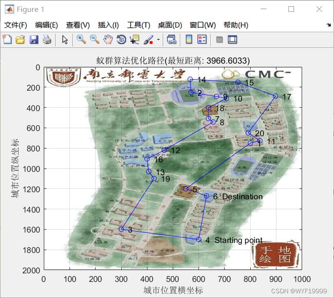
title(['蚁群算法优化路径(最短距离: ' num2str(shortest_Length) ')'])
figure(2)
plot(1: NC_max, lAverage ,'bo', 1:NC_max, lBest, 'mo:')
legend('平均距离','最短距离')
xlabel('迭代次数')
ylabel('距离')
title('蚁群算法各代最短距离与平均距离对比')
结果展示


3.遗传算法
流程图

代码
%% 1.清空环境变量
clear all;
clc;

%% (可选)读入背景南邮地图
img = imread('C:\Users\wyf\Desktop\map.png');
% 设置图片在绘制时的尺寸,估测的南邮仙林校区大小
min_x = 0;
max_x = 1000;
min_y = 0;
max_y = 2000;
%插入背景图
imagesc([min_x max_x], [min_y max_y], flip(img,3));

%% 2.导入数据
load citys_data.mat;          %数据集的变量名为citys

%% 3.计算城市间相互距离
n=size(citys,1);
D=zeros(n,n);

for i=1:n
    for j=i+1:n
        D(i,j)=sqrt(sum((citys(i,:)-citys(j,:)).^2));
        D(j,i)=D(i,j);
    end
end

%% 4.初始化参数
m=2000;                         %种群个数
pop=zeros(m,n);                 %种群
crospro=0.8;                    %交叉概率
mutpro=0.1;                     %变异概率
gen=1;                          %迭代计数器
genmax=2000;                    %最大迭代次数
fitness=zeros(m,1);             %适应度函数值
Route_best=zeros(genmax,n);     %各代最佳路径
Length_best=zeros(genmax,1);    %各代最佳路径的长度
Length_ave=zeros(genmax,1);     %各代路径的平均长度

%% 5.产生初始种群
tic
% 5.1随机产生初始种群
for i=1:m
    pop(i,:)=randperm(n);
end

% 5.2计算初始种群适应度函数值
for i=1:m
    for j=1:n-1
        fitness(i)=fitness(i) + D(pop(i,j),pop(i,j+1));
    end
    fitness(i)=fitness(i) + D(pop(i,end),pop(i,1));
end

% 5.3计算最短路径及平均距离
[min_Length,min_index]=min(fitness);
Length_best(1)=min_Length;
Route_best(1,:)=pop(min_index,:);
Length_ave(1)=mean(fitness);

%% 6.迭代寻找最佳路径
while gen<=genmax
    % 6.1更新迭代次数
    gen=gen+1;

    % 6.2选择算子(轮盘赌法)
    P=1./fitness;
    P=P/sum(P);        %计算每一个城市的概率
    Pc=cumsum(P);      %计算累积概率

    popnew=zeros(m,n);
    for i=1:m
        target_index=find(Pc>=rand);
        target=pop(target_index(1),:);
        popnew(i,:)=target;
    end

    % 6.3交叉算子(部分匹配交叉)
    for i=1:2:n   %两两之间相互交叉
        if crospro>rand  %判断是否进行交叉
            child1path=zeros(1,n);
            child2path=zeros(1,n);

            setsize=floor(n/2)-1;      %匹配区域城市的数量
            offset1=randi(setsize);    %匹配区域的下边界
            offset2=offset1+setsize-1; %匹配区域的上边界

            %匹配区域
            for j=offset1:offset2
                child1path(j)=popnew(i+1,j);
                child2path(j)=popnew(i,j);
            end

            % 非匹配区域
            for j=1:offset1-1
                child1path(j)=popnew(i,j);
                child2path(j)=popnew(i+1,j);
            end

            for j=offset2+1:n
                child1path(j)=popnew(i,j);
                child2path(j)=popnew(i+1,j);
            end

            % 子代1冲突检测
            for j=offset1:offset2
                if ~ismember(child1path(j),popnew(i,offset1:offset2)) %不在交叉段内
                    %寻找映射关系
                    a1=child1path(j);
                    a2=popnew(i,j);
                    while ismember(a2,child1path(offset1:offset2))
                        temp_index=find(popnew(i+1,:)==a2);
                        a1=a2;
                        a2=popnew(i,temp_index);
                    end
                    %寻找重复数字位置
                    b1=find(child1path==child1path(j));
                    if length(b1)>1
                        if b1(1)>offset2||b1(1)<offset1
                            change_index=b1(1);
                        else
                            change_index=b1(2);
                        end
                    end
                    %替代重复数字
                    child1path(change_index)=a2;
                end
            end

            % 子代2冲突检测(同上)
            for j=offset1:offset2
                if ~ismember(child2path(j),popnew(i+1,offset1:offset2)) %不在交叉段内
                    %寻找映射关系
                    a1=child2path(j);
                    a2=popnew(i+1,j);
                    while ismember(a2,child2path(offset1:offset2))
                        temp_index=find(popnew(i,:)==a2);
                        a1=a2;
                        a2=popnew(i+1,temp_index);
                    end
                    %寻找重复数字位置
                    b2=find(child2path==child2path(j));
                    if length(b2)>1
                        if b2(1)>offset2||b2(1)<offset1
                            change_index=b2(1);
                        else
                            change_index=b2(2);
                        end
                    end
                    %替代重复数字
                    child2path(change_index)=a2;
                end
            end

            popnew(i,:)=child1path;
            popnew(i+1,:)=child2path;
        end
    end

    % 6.4变异算子
    for i=1:m
        if mutpro>rand %判断是否变异
            %随机抽两个数字
            y=round(rand(1,2)*(n-1)+1);
            %交换位置
            temp=popnew(i,y(1));
            popnew(i,y(1))=popnew(i,y(2));
            popnew(i,y(2))=temp;
        end
    end

    % 6.5计算新一代种群适应度函数值
    pop=popnew;
    fitness=zeros(m,1);
    for i=1:m
        for j=1:n-1
            fitness(i)=fitness(i) + D(pop(i,j),pop(i,j+1));
        end
        fitness(i)=fitness(i) + D(pop(i,end),pop(i,1));
    end

    % 6.6计算最短路径及平均距离
    [min_Length,min_index]=min(fitness);
    Length_ave(gen)=mean(fitness);
    if min_Length<Length_best(gen-1)
        Length_best(gen)=min_Length;
        Route_best(gen,:)=pop(min_index,:);
    else
        Length_best(gen)=Length_best(gen-1);
        Route_best(gen,:)=Route_best(gen-1,:);
    end

end
toc
%% 7.结果显示
best_route=Route_best(end,:);
best_length=Length_best(end,:);
disp(['最短距离: ' num2str(best_length)]);
disp(['最短路径: ' num2str(best_route)]);

%% 8.绘图
hold on
figure(1)
plot([citys(best_route,1);citys(best_route(1),1)],[citys(best_route,2);citys(best_route(1),2)],'bo-')
for i=1:size(citys,1)
    text(citys(i,1),citys(i,2),[' ' num2str(i)]);
end
text(citys(best_route(1),1),citys(best_route(1),2),'     Starting point');
text(citys(best_route(end),1),citys(best_route(end),2),'     Destination');
xlabel('城市位置横坐标')
ylabel('城市位置纵坐标')
title(['遗传算法优化路径(最短距离:' num2str(best_length) ')'])

figure(2)
plot(1:genmax+1,Length_ave,'bo:',1:genmax+1,Length_best,'mo')
legend('平均距离','最短距离')
xlabel('迭代次数')
ylabel('距离')
title('遗传算法各代最短距离与平均距离对比')
结果展示


4.粒子群算法
流程图

代码
%% 1.清空环境变量
clear all;
clc;
%% (可选)读入背景南邮地图
img = imread('C:\Users\wyf\Desktop\map.png');
% 设置图片在绘制时的尺寸,估测的南邮仙林校区大小
min_x = 0;
max_x = 1000;
min_y = 0;
max_y = 2000;
%插入背景图
imagesc([min_x max_x], [min_y max_y], flip(img,3));
%% 2.导入数据
load citys_data.mat; %数据集的变量名为citys
%% 3.计算城市间相互距离
n=size(places,1);
D=zeros(n,n);
for i=1:n
for j=i+1:n
D(i,j)=sqrt(sum((places(i,:)-places(j,:)).^2));
D(j,i)=D(i,j);
end
end
%% 4.初始化参数
c1=0.1; %个体学习因子
c2=0.075; %社会学习因子
w=1; %惯性因子
m=500; %粒子数量
pop=zeros(m,n); %粒子位置
v=zeros(m,n); %粒子速度
gen=1; %迭代计数器
genmax=1000; %迭代次数
fitness=zeros(m,1); %适应度函数值
Pbest=zeros(m,n); %个体极值路径
Pbest_fitness=zeros(m,1); %个体极值
Gbest=zeros(genmax,n); %群体极值路径
Gbest_fitness=zeros(genmax,1); %群体极值
Length_ave=zeros(genmax,1); %各代路径的平均长度
ws=1; %惯性因子最大值
we=0.8; %惯性因子最小值
%% 5.产生初始粒子
tic
% 5.1随机产生粒子初始位置和速度
for i=1:m
pop(i,:)=randperm(n);
v(i,:)=randperm(n);
end
% 5.2计算粒子适应度函数值
for i=1:m
for j=1:n-1
fitness(i)=fitness(i) + D(pop(i,j),pop(i,j+1));
end
fitness(i)=fitness(i) + D(pop(i,end),pop(i,1));
end
% 5.3计算个体极值和群体极值
Pbest_fitness=fitness;
Pbest=pop;
[Gbest_fitness(1),min_index]=min(fitness);
Gbest(1,:)=pop(min_index,:);
Length_ave(1)=mean(fitness);
%% 6.迭代寻优
while gen<genmax
% 6.1更新迭代次数与惯性因子
gen=gen+1;
w = ws - (ws-we)*(gen/genmax)^2;
% 6.2更新速度
%个体极值修正部分
change1=position_minus_position(Pbest,pop);
change1=constant_times_velocity(c1,change1);
%群体极值修正部分
change2=position_minus_position(repmat(Gbest(gen-1,:),m,1),pop);
change2=constant_times_velocity(c2,change2);
%原速度部分
v=constant_times_velocity(w,v);
%修正速度
for i=1:m
for j=1:n
if change1(i,j)~=0
v(i,j)=change1(i,j);
end
if change2(i,j)~=0
v(i,j)=change2(i,j);
end
end
end
% 6.3更新位置
pop=position_plus_velocity(pop,v);
% 6.4适应度函数值更新
fitness=zeros(m,1);
for i=1:m
for j=1:n-1
fitness(i)=fitness(i) + D(pop(i,j),pop(i,j+1));
end
fitness(i)=fitness(i) + D(pop(i,end),pop(i,1));
end
% 6.5个体极值与群体极值更新
for i=1:m
if fitness(i)<Pbest_fitness(i)
Pbest_fitness(i)=fitness(i);
Pbest(i,:)=pop(i,:);
end
end
[minvalue,min_index]=min(fitness);
if minvalue<Gbest_fitness(gen-1)
Gbest_fitness(gen)=minvalue;
Gbest(gen,:)=pop(min_index,:);
else
Gbest_fitness(gen)=Gbest_fitness(gen-1);
Gbest(gen,:)=Gbest(gen-1,:);
end
Length_ave(gen)=mean(fitness);
end
toc
%% 7.结果显示
[Shortest_Length,index] = min(Gbest_fitness);
Shortest_Route = Gbest(index,:);
disp(['最短距离:' num2str(Shortest_Length)]);
disp(['最短路径:' num2str([Shortest_Route Shortest_Route(1)])]);
%% 8.绘图
hold on
figure(1)
plot([places(Shortest_Route,1);places(Shortest_Route(1),1)],...
[places(Shortest_Route,2);places(Shortest_Route(1),2)],'bo-');
grid on
for i = 1:size(places,1)
text(places(i,1),places(i,2),[' ' num2str(i)]);
end
text(places(Shortest_Route(1),1),places(Shortest_Route(1),2),' Starting point');
text(places(Shortest_Route(end),1),places(Shortest_Route(end),2),' Destination');
xlabel('城市位置横坐标')
ylabel('城市位置纵坐标')
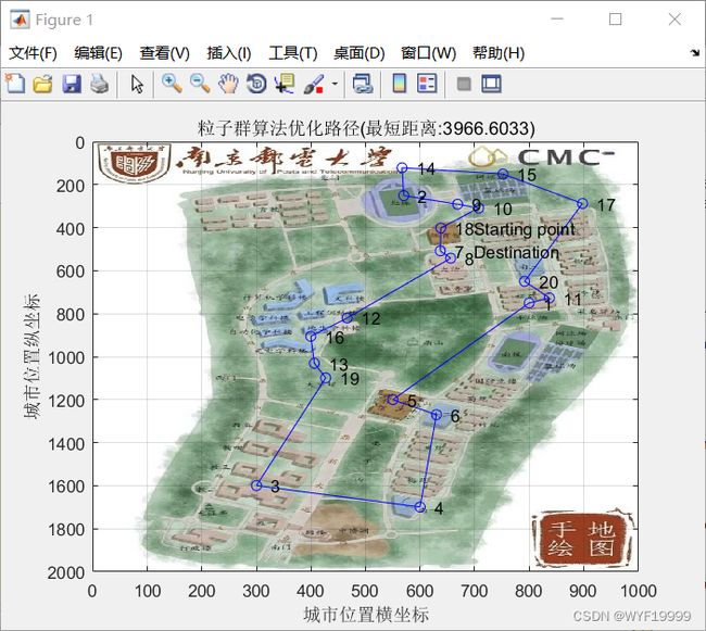
title(['粒子群算法优化路径(最短距离:' num2str(Shortest_Length) ')'])
figure(2)
plot(1:genmax,Length_ave,'bo',1:genmax,Gbest_fitness,'mo:')
legend('平均距离','最短距离')
xlabel('迭代次数')
ylabel('距离')
title('粒子群算法各代最短距离与平均距离对比')
结果展示