吴恩达《Machine Learning》-machine-learning-ex1线性回归作业（一）

ex1.m

  %% Machine Learning Online Class - Exercise 1: Linear Regression
    
    %  Instructions
    %  ------------
    %
    %  This file contains code that helps you get started on the
    %  linear exercise. You will need to complete the following functions
    %  in this exericse:
    %
    %     warmUpExercise.m
    %     plotData.m
    %     gradientDescent.m
    %     computeCost.m
    %     gradientDescentMulti.m
    %     computeCostMulti.m
    %     featureNormalize.m
    %     normalEqn.m
    %
    %  For this exercise, you will not need to change any code in this file,
    %  or any other files other than those mentioned above.
    %
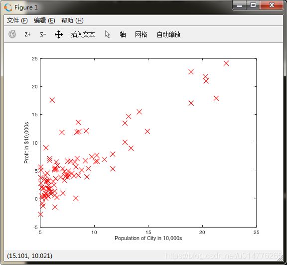
    % x refers to the population size in 10,000s
    % y refers to the profit in $10,000s
    %
    
    %% Initialization
    clear ; close all; clc
    
    %% ==================== Part 1: Basic Function ====================
    % Complete warmUpExercise.m
    fprintf('Running warmUpExercise ... \n');
    fprintf('5x5 Identity Matrix: \n');
    warmUpExercise()
    
    fprintf('Program paused. Press enter to continue.\n');
    pause;
    
    
    %% ======================= Part 2: Plotting =======================
    fprintf('Plotting Data ...\n')
    data = load('ex1data1.txt');
    X = data(:, 1); y = data(:, 2);
    m = length(y); % number of training examples
    
    % Plot Data
    % Note: You have to complete the code in plotData.m
    plotData(X, y);
    
    fprintf('Program paused. Press enter to continue.\n');
    pause;
    
    %% =================== Part 3: Cost and Gradient descent ===================
    
    X = [ones(m, 1), data(:,1)]; % Add a column of ones to x
    theta = zeros(2, 1); % initialize fitting parameters
    
    % Some gradient descent settings
    iterations = 1500;
    alpha = 0.01;
    
    fprintf('\nTesting the cost function ...\n')
    % compute and display initial cost
    J = computeCost(X, y, theta);
    fprintf('With theta = [0 ; 0]\nCost computed = %f\n', J);
    fprintf('Expected cost value (approx) 32.07\n');
    
    % further testing of the cost function
    J = computeCost(X, y, [-1 ; 2]);
    fprintf('\nWith theta = [-1 ; 2]\nCost computed = %f\n', J);
    fprintf('Expected cost value (approx) 54.24\n');
    
    fprintf('Program paused. Press enter to continue.\n');
    pause;
    
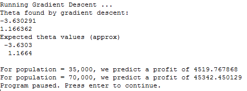
    fprintf('\nRunning Gradient Descent ...\n')
    % run gradient descent
    theta = gradientDescent(X, y, theta, alpha, iterations);
    
    % print theta to screen
    fprintf('Theta found by gradient descent:\n');
    fprintf('%f\n', theta);
    fprintf('Expected theta values (approx)\n');
    fprintf(' -3.6303\n  1.1664\n\n');
    
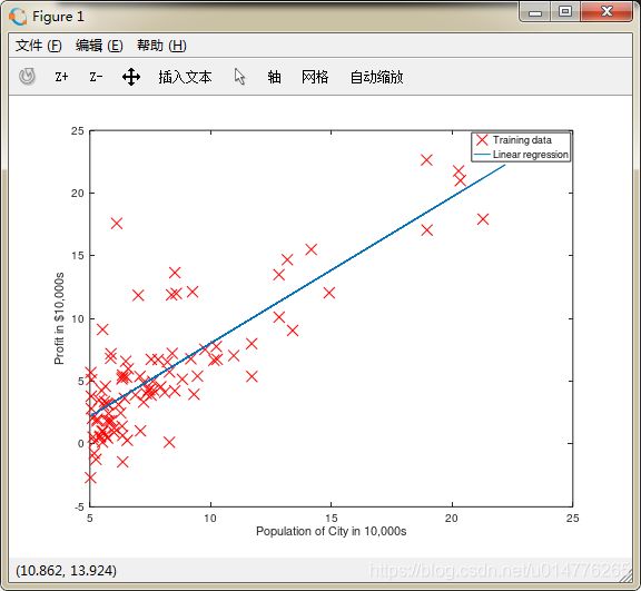
    % Plot the linear fit
    hold on; % keep previous plot visible
    plot(X(:,2), X*theta, '-')
    legend('Training data', 'Linear regression')
    hold off % don't overlay any more plots on this figure
    
    % Predict values for population sizes of 35,000 and 70,000
    predict1 = [1, 3.5] *theta;
    fprintf('For population = 35,000, we predict a profit of %f\n',...
        predict1*10000);
    predict2 = [1, 7] * theta;
    fprintf('For population = 70,000, we predict a profit of %f\n',...
        predict2*10000);
    
    fprintf('Program paused. Press enter to continue.\n');
    pause;
    
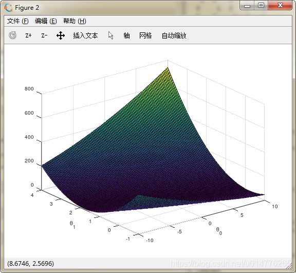
    %% ============= Part 4: Visualizing J(theta_0, theta_1) =============
    fprintf('Visualizing J(theta_0, theta_1) ...\n')
    
    % Grid over which we will calculate J
    theta0_vals = linspace(-10, 10, 100);
    theta1_vals = linspace(-1, 4, 100);
    
    % initialize J_vals to a matrix of 0's
    J_vals = zeros(length(theta0_vals), length(theta1_vals));
    
    % Fill out J_vals
    for i = 1:length(theta0_vals)
        for j = 1:length(theta1_vals)
    	  t = [theta0_vals(i); theta1_vals(j)];
    	  J_vals(i,j) = computeCost(X, y, t);
        end
    end
    
    
    % Because of the way meshgrids work in the surf command, we need to
    % transpose J_vals before calling surf, or else the axes will be flipped
    J_vals = J_vals';
    % Surface plot
    figure;
    surf(theta0_vals, theta1_vals, J_vals)
    xlabel('\theta_0'); ylabel('\theta_1');
    
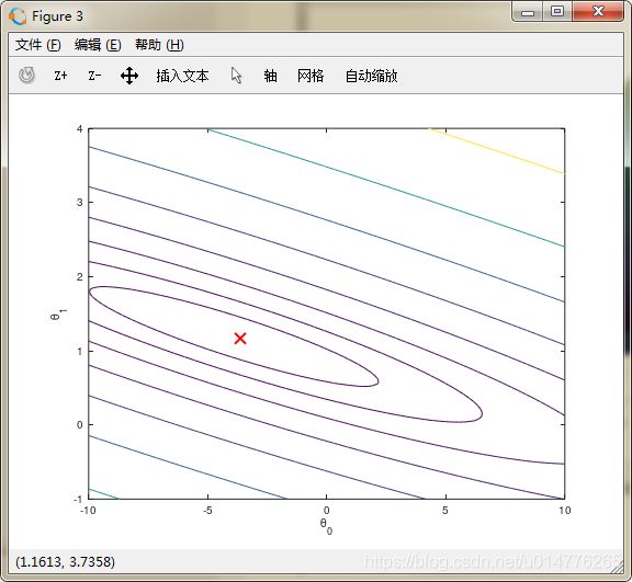
    % Contour plot
    figure;
    % Plot J_vals as 15 contours spaced logarithmically between 0.01 and 100
    contour(theta0_vals, theta1_vals, J_vals, logspace(-2, 3, 20))
    xlabel('\theta_0'); ylabel('\theta_1');
    hold on;
    plot(theta(1), theta(2), 'rx', 'MarkerSize', 10, 'LineWidth', 2);

显示J（θ）

plotData.m数据集画图函数

function plotData(x, y)
%PLOTDATA Plots the data points x and y into a new figure 
%   PLOTDATA(x,y) plots the data points and gives the figure axes labels of
%   population and profit.

figure; % open a new figure window

% ====================== YOUR CODE HERE ======================
% Instructions: Plot the training data into a figure using the 
%               "figure" and "plot" commands. Set the axes labels using
%               the "xlabel" and "ylabel" commands. Assume the 
%               population and revenue data have been passed in
%               as the x and y arguments of this function.
%
% Hint: You can use the 'rx' option with plot to have the markers
%       appear as red crosses. Furthermore, you can make the
%       markers larger by using plot(..., 'rx', 'MarkerSize', 10);

plot(x, y, 'rx', 'MarkerSize', 10); % Plot the data
ylabel('Profit in $10,000s'); % Set the y†axis label
xlabel('Population of City in 10,000s'); % Set the xxaxis label



% ============================================================

end

数据集图片

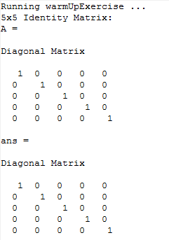
warmUpExercise.m 画出对角矩阵

function A = warmUpExercise()
%WARMUPEXERCISE Example function in octave
%   A = WARMUPEXERCISE() is an example function that returns the 5x5 identity matrix

A = [];
% ============= YOUR CODE HERE ==============
% Instructions: Return the 5x5 identity matrix 
%               In octave, we return values by defining which variables
%               represent the return values (at the top of the file)
%               and then set them accordingly. 


A = eye(5)


% ===========================================


end

运行结果：

computeCost.m 计算损失函数

公式：

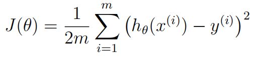
function J = computeCost(X, y, theta)
%COMPUTECOST Compute cost for linear regression
%   J = COMPUTECOST(X, y, theta) computes the cost of using theta as the
%   parameter for linear regression to fit the data points in X and y

% Initialize some useful values
m = length(y); % number of training examples

% You need to return the following variables correctly 
J = 0;

% ====================== YOUR CODE HERE ======================
% Instructions: Compute the cost of a particular choice of theta
%               You should set J to the cost.

    h = X*theta;
    difference = h - y;
    J = sum(difference.^2)/(2*m);



% =========================================================================

end

运行结果：

gradientDescent.m 梯度下降

公式：

function [theta, J_history] = gradientDescent(X, y, theta, alpha, num_iters)
%GRADIENTDESCENT Performs gradient descent to learn theta
%   theta = GRADIENTDESCENT(X, y, theta, alpha, num_iters) updates theta by 
%   taking num_iters gradient steps with learning rate alpha

% Initialize some useful values
m = length(y); % number of training examples
J_history = zeros(num_iters, 1);

for iter = 1:num_iters

    % ====================== YOUR CODE HERE ======================
    % Instructions: Perform a single gradient step on the parameter vector
    %               theta. 
    %
    % Hint: While debugging, it can be useful to print out the values
    %       of the cost function (computeCost) and gradient here.
    %


     H = X * theta;
    theta = theta - (alpha * 1.0) / m .* (X' * (H - y));



    % ============================================================

    % Save the cost J in every iteration    
    J_history(iter) = computeCost(X, y, theta);

end

end

运行结果：