简单的二层BP神经网络-实现逻辑与门（Matlab和Python）

该程序主要是设计一个2层的神经网络，通过BP算法实现与门逻辑。

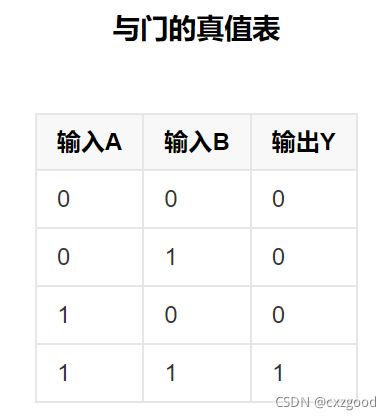
一、逻辑与门

二、二层的神经网络

三、数学推导

根据真值表可知，输入输出的对应逻辑关系。

故设输入X,输出Y为

            

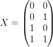
权值W1为2*2矩阵,W2为2*1矩阵

(1).  前向计算过程

第1个神经元输出为：

第2个神经元输出为：

其中：

(2).  反向传播过程

公式由链式求导法则得出，这里不做推导。结果如下：

第2个神经元误差为：

第1个神经元误差为：

其中：

权值W2的偏导数为：

权值W1的偏导数为：

(3).  梯度下降算法更新权值

 

四、程序  

Matlab代码：

clear all;clc
%数据初始化
X = [0 0;0 1; 1 0;1 1];
Y = [0;0;0;1];
w1 = 3 * rand(2,2) - 0.5;
w2 = 3 * rand(2,1) - 0.5;
W1 = w1;
W2 = w2;
m = length(Y);
alpha = 5;                 %learning_rate
number_iters = 50000;      %number_of_training_iterations

%迭代
for i=1:number_iters
  %Forward Propagation
   a0 = X;                        %4*2
   a1 = X * W1;                   %4*2
   z1 = sigmoid(a1);              %4*2
   a2 = z1 * W2;                  %4*1
   z2 = sigmoid(a2);              %4*1
   
  %Back Propagation
   error2 = Y - z2;                         %4*1
   delta2 = error2.* sigmoidGradient(a2);   %4*1
   error1 = delta2 * W2';                   %4*2
   delta1 = error1.* sigmoidGradient(a1);   %4*2
   
   W1_adjustment = X' * delta1;             %2*2
   W2_adjustment = z1' * delta2;            %2*1
   W1 = W1 + alpha * W1_adjustment;         %2*2
   W2 = W2 + alpha * W2_adjustment;         %2*1
   
  %Cost Function
   J(i) = (1/m) * sum(Y - z2)^2;   
end

%绘制代价函数曲线
plot(J);
xlabel('number of iterations')
ylabel('Costfunction in the output layer');

%输出随机初始值
fprintf('Stage 1) Random starting synaptic weights:\n');
disp(w1);

disp(w2);

%输出训练后参数值
fprintf('Stage 2) New synaptic weights after training:\n');
disp(W1);

disp(W2);

%预测
fprintf('Stage 3) Considering a new situation [0 0;0 1; 1 0;1 1] -> ?:\n');
x = [0 0;0 1; 1 0;1 1];   
y = sigmoid(sigmoid(x * W1) * W2);

%取整
% [a,b]=size(y);
% for i=1:a
%     for j=1:b
%         if y(i,j)>0.5
%             y(i,j)=1;
%         else y(i,j)=0;
%         end
%     end
% end

disp(y);

输出结果：

Stage 3) Considering a new situation [0 0;0 1; 1 0;1 1] -> ?:
    0.0002
    0.0044
    0.0056
    0.9950

代价函数图像：

Python代码：

from matplotlib import pyplot as plt
from numpy import exp, array, random, dot


class NeuronLayer():
    def __init__(self, number_of_neurons, number_of_inputs_per_neuron):
        self.synaptic_weights = 3 * random.random((number_of_inputs_per_neuron, number_of_neurons)) - 0.5


class NeuralNetwork():
    def __init__(self, layer1, layer2):
        self.layer1 = layer1
        self.layer2 = layer2

        self.learning_rate = 10
    # The Sigmoid function, which describes an S shaped curve.
    # We pass the weighted sum of the inputs through this function to
    # normalise them between 0 and 1.
    def __sigmoid(self, x):
        return 1 / (1 + exp(-x))

    # The derivative of the Sigmoid function.
    # This is the gradient of the Sigmoid curve.
    # It indicates how confident we are about the existing weight.
    def __sigmoid_derivative(self, x):
        return x * (1 - x)

    # We train the neural network through a process of trial and error.
    # Adjusting the synaptic weights each time.
    def train(self, training_set_inputs, training_set_outputs, number_of_training_iterations):
        for iteration in range(number_of_training_iterations):
            # Pass the training set through our neural network
            output_from_layer_1, output_from_layer_2 = self.think(training_set_inputs)

            # Calculate the error for layer 2 (The difference between the desired output
            # and the predicted output).
            layer2_error = training_set_outputs - output_from_layer_2
            layer2_delta = layer2_error * self.__sigmoid_derivative(output_from_layer_2)

            # Calculate the error for layer 1 (By looking at the weights in layer 1,
            # we can determine by how much layer 1 contributed to the error in layer 2).
            layer1_error = layer2_delta.dot(self.layer2.synaptic_weights.T)
            layer1_delta = layer1_error * self.__sigmoid_derivative(output_from_layer_1)

            # Calculate how much to adjust the weights by
            layer1_adjustment = training_set_inputs.T.dot(layer1_delta)
            layer2_adjustment = output_from_layer_1.T.dot(layer2_delta)

            # Adjust the weights.
            self.layer1.synaptic_weights += layer1_adjustment * self.learning_rate
            self.layer2.synaptic_weights += layer2_adjustment * self.learning_rate



    # The neural network thinks.
    def think(self, inputs):
        output_from_layer1 = self.__sigmoid(dot(inputs, self.layer1.synaptic_weights))
        output_from_layer2 = self.__sigmoid(dot(output_from_layer1, self.layer2.synaptic_weights))
        return output_from_layer1, output_from_layer2

    # The neural network prints its weights
    def print_weights(self):
        print("    Layer 1 (2 neurons, each with 2 inputs):")
        print(self.layer1.synaptic_weights)
        print("    Layer 2 (1 neuron, with 2 inputs):")
        print(self.layer2.synaptic_weights)

if __name__ == "__main__":

    #Seed the random number generator
#    random.seed(2)

    # Create layer 1 (2 neurons, each with 2 inputs)
    layer1 = NeuronLayer(2, 2)

    # Create layer 2 (a single neuron with 2 inputs)
    layer2 = NeuronLayer(1, 2)

    # Combine the layers to create a neural network
    neural_network = NeuralNetwork(layer1, layer2)


    print("Stage 1) Random starting synaptic weights: ")
    neural_network.print_weights()

    # The training set. We have 4 examples, each consisting of 2 input values
    # and 1 output value.
    training_set_inputs = array([[0, 0], [0, 1], [1, 0], [1, 1]])
    training_set_outputs = array([[0, 0, 0, 1]]).T

    # Train the neural network using the training set.
    # Do it 60,000 times and make small adjustments each time.
    neural_network.train(training_set_inputs, training_set_outputs, 60000)

    print("Stage 2) New synaptic weights after training: ")
    neural_network.print_weights()

    # Test the neural network with a new situation.
    print("Stage 3) Considering a new situation [0,1] -> ?: ")
    hidden_state, output = neural_network.think(array([0, 1]))
    print(output)
 

输出结果：

Stage 3) Considering a new situation [ , ] -> ?: 
[9.78921931e-05]
[0.00284118]
[0.0036443]
[0.99679971]

五、总结

BP神经网络作为最基础的机器学习之一，是机器学习初学者的必经之路。作者在学习的过程中，得到很多前辈们的经验帮助，特此将代码整理出来，反馈于各位。

注：代码来源于网络搜集及自己的修改，如侵可删。