基于单位四元数的姿态插补算法

基于单位四元数的姿态插补算法

摘要

现代制造领域对工业机器人的需求越来越多，对工业机器人性能要求也越来越苛刻。机器人运动轨迹插补算法是决定机器人性能的核心技术之一，直接影响着机器人的运动精度、速度和平滑性等主要性能。在曲面、曲线加工，喷涂、弧焊等领域，机器人的轨迹插补，尤其是姿态插补对加工质量和加工效率起到决定性作用。目前对机器人的姿态描述主要使用欧拉法，此类方法存在奇异性以及角速度耦合等问题。单位四元数对姿态的描述更加自然，另外还有效避免了欧拉角旋转时奇异性的问题，且基于单位四元数的运动插补算法计算效率要比欧拉角和余弦矩阵高。目前，单位四元数已经在航天器姿态控，动画制作以及 CAD三维建模等多个领域有着广泛的应用。本文研究的算法等材料可以在gihub下载-链接

单位四元数空间与欧式空间的转化

构造姿态曲线的主要问题在于在单位四元数空间中的姿态曲线的构造问题。因为单位四元数存在于${\mathbf{S}}^3$ 空间中，然而欧式空间中的度量并不适用于${\mathbf{S}}^3$ 空间。同时在欧氏空间中位移的导数为速度，而${\mathbf{S}}^3$ 空间中四元数的导数不是角速度，而是角速度与四元数本身的乘积: $q^{\prime }=\omega q/2$. 下面研究将单位四元数曲线构造问题转换为在欧氏空间中单位矢量的球面曲线构造问题。

四元数的旋转变换表示空间定点旋转

定理: 设$q$和$R$为非标量四元数，如果令
$$q=|\mathbf{E}|(cos\frac{\alpha }{2}+\frac{\mathbf{E}}{|\mathbf{E}|}sin\frac{\alpha }{2})$$
则
$$R^{\prime }=q\ast R\ast q^{-1}$$
是四元数，其范数和标量与四元数$R$相同，其矢量部分Vect $R^{\prime }$为Vect $R$绕欧拉轴$\mathbf{E}$旋转$\alpha$角。因此，绕定点矢量旋转可以用四元数变换来表示。

注意q是单位四元数，可表示为
$$q=q_0+q_1\mathbf{i}+q_2\mathbf{j}+q_3\mathbf{k}=cos\frac{\alpha }{2}+\omega sin\frac{\alpha }{2}$$
其中$\omega$是单位矢量。

为什么四元数可以表示坐标系旋转变换？因为坐标系是由三个单位矢量构成的，上面定理发现，四元数可以对矢量进行旋转变换，对坐标系做旋转变换可以看成是对坐标系的三个单位矢量做旋转变换。

因为表示一个旋转变换可以用一个欧拉轴的单位矢量$\omega$和一个角度$\alpha$来描述，有的书称为等效轴表示法。而这里$\omega$是个定值，对该旋转变换进行插补时，只需对角度$\theta$进行插补即可，而四元数又是联系这两个参数和旋转变换矩阵表示的桥梁，可以把中间插补姿态转化为旋转矩阵。

四元数和旋转矩阵的关系如下：

已知旋转矩阵计算四元数
$$R=\left[\begin{array}{ccc}{r}_{11}& r_{12}& r_{13}\\ r_{21}& r_{22}& r_{23}\\ r_{31}& r_{32}& r_{33}\end{array}\right]$$
对应的等效轴参数为

（1）若(trR-1)/2=1(即为单位阵),那么$\alpha =0$, $\omega$未定义。

（2）若trR=-1,那么$\alpha =\pi$, $\omega$的解为以下可行的向量
$$\omega =\frac{1}{\sqrt{2(1+r_{33})}}\left[\begin{array}{c}{r}_{13}\\ r_{23}\\ 1+r_{33}\end{array}\right]$$
或者
$$\omega =\frac{1}{\sqrt{2(1+r_{22})}}\left[\begin{array}{c}{r}_{12}\\ 1+r_{22}\\ r_{32}\end{array}\right]$$
或者
$$\omega =\frac{1}{\sqrt{2(1+r_{11})}}\left[\begin{array}{c}1+r_{11}\\ r_{21}\\ r_{31}\end{array}\right]$$
(3)否则，$\alpha =co{s}^{-1}(\frac{1}{2}(trR-1)\in (0,\pi )$,且
$$\omega =\frac{1}{2\text{sin}\alpha }\left[\begin{array}{c}{r}_{32}-r_{23}\\ r_{13}-r_{31}\\ r_{21}-r_{12}\end{array}\right]$$
那么对应的四元数为
$$q_0=\text{cos}\frac{\alpha }{2},q_1=\frac{r_{32}-r_{23}}{2\text{sin}\alpha },q_2=\frac{r_{13}-r_{31}}{2\text{sin}\alpha },q_3=\frac{r_{21}-r_{12}}{2\text{sin}\alpha }$$
已知四元数计算旋转矩阵
$$R=\left[\begin{array}{ccc}{q}_0^2+q_1^2-q_2^2-q_3^2& 2(q_1{q}_2-q_0{q}_3)& 2(q_0{q}_2+q_1{q}_3)\\ 2(q_0{q}_3+q_1{q}_2)& q_0^2-q_1^2+q_2^2-q_3^2& 2(q_2{q}_3-q_0{q}_1)\\ 2(q_1{q}_3-q_0{q}_2)& 2(q_0{q}_1+q_2{q}_3)& q_0^2-q_1^2-q_2^2+q_3^2\end{array}\right]$$
上面旋转矩阵与欧拉轴，转角，四元数之间的相互转换，我们写成以下三个函数模块，后面构建姿态插补算法将会用到它们。C语言实现代码如下：

	#define			PI					3.14159265358979323846
	//if the norm of vector is near zero(< 1.0E-6),regard as zero.
	#define			ZERO_VECTOR			1.0E-6	
	#define			ZERO_ELEMENT		1.0E-6		
	#define			ZERO_ANGLE			1.0E-6
	#define			ZERO_DISTANCE		1.0E-6
	#define			ZERO_VALUE			1.0E-6
/**
 * @brief 			Description: Computes the unit vector of Euler axis and rotation angle corresponding to rotation matrix.
 * @param[in]		R				A rotation matrix.
 * @param[out]		omghat			the unit vector of Euler axis .
 * @param[out]		theta			the rotation angle.
 * @return			No return value.
 * @retval			0
 * @note:			if  theta is zero ,the unit axis is undefined and set it as a zero vector [0;0;0].
 *@warning:
*/
void RotToAxisAng(double R[3][3],double omghat[3],double *theta)
{
	double tmp;
	double omg[3] = { 0 };
	double acosinput = (R[0][0] + R[1][1] + R[2][2] - 1.0) / 2.0;
	if (fabs(acosinput-1.0)<ZERO_VALUE)
	{
		memset(omghat, 0, 3 * sizeof(double));
		*theta = 0.0;
	}
	else if (acosinput <= -1.0)
	{
		if ((1.0 + R[2][2]) >= ZERO_VALUE)
		{
			omg[0] = 1.0 / sqrt(2 * (1.0 + R[2][2]))*R[0][2];
			omg[1] = 1.0 / sqrt(2 * (1.0 + R[2][2]))*R[1][2];
			omg[2] = 1.0 / sqrt(2 * (1.0 + R[2][2]))*(1.0 + R[2][2]);
		}
		else if ((1.0 + R[1][1] >= ZERO_VALUE))
		{
			omg[0] = 1.0 / sqrt(2 * (1.0 + R[1][1]))*R[0][1];
			omg[1] = 1.0 / sqrt(2 * (1.0 + R[1][1]))*(1.0 + R[1][1]);
			omg[2] = 1.0 / sqrt(2 * (1.0 + R[1][1]))*R[2][1];
		}
		else
		{
			omg[0] = 1.0 / sqrt(2 * (1.0 + R[0][0]))*(1.0 + R[0][0]);
			omg[1] = 1.0 / sqrt(2 * (1.0 + R[0][0]))*R[1][0];
			omg[2] = 1.0 / sqrt(2 * (1.0 + R[0][0]))*R[2][0];
		}
		omghat[0] = omg[0];
		omghat[1] = omg[1];
		omghat[2] = omg[2];
		*theta=PI;
	}
	else
	{
		*theta = acos(acosinput);
		tmp = 2.0*sin(*theta);
		omghat[0] = (R[2][1] - R[1][2]) / tmp;
		omghat[1] = (R[0][2] - R[2][0]) / tmp;
		omghat[2] = (R[1][0] - R[0][1]) / tmp;

	}

	return;
}


/**
 * @brief 			Description: Computes the unit quaternion corresponding to the Euler axis and rotation angle.
 * @param[in]		omg				Unit vector of Euler axis.
 * @param[in]		theta			Rotation angle.
 * @param[in]		q				The unit quaternion
 * @return			No return value.
 * @note:
 *@warning:
*/
void AxisAngToQuaternion(double omg[3],double theta, double q[4])
{
	q[0] = cos(theta / 2.0);
	q[1] = omg[0] * sin(theta / 2.0);
	q[2] = omg[1] * sin(theta / 2.0);
	q[3] = omg[2] * sin(theta / 2.0);
	return;
}


/**
 * @brief 			Description:Computes the unit quaternion corresponding to a rotation matrix.
 * @param[in]		q				Unit quaternion.
 * @param[out]		R				Rotation matrix.
 * @return			No return value.
 * @note:
 * @warning:
*/
void QuaternionToRot(double q[4], double R[3][3])
{
	R[0][0] = q[0] * q[0] - q[1] * q[1] - q[2] * q[2] - q[3] * q[3];
	R[0][1] = 2.0*(q[1] * q[2] - q[0] * q[3]);
	R[0][2] = 2.0*(q[0] * q[2] + q[1] * q[3]);
	R[1][0] = 2.0*(q[0] * q[3] + q[1] * q[2]);
	R[1][1] = q[0] * q[0] - q[1] * q[1] + q[2] * q[2] - q[3] * q[3];
	R[1][2] = 2.0*(q[2] * q[3] - q[0] * q[1]);
	R[2][0] = 2.0*(q[1] * q[3] - q[0] * q[2]);
	R[2][1] = 2.0*(q[0] * q[1] + q[2] * q[3]);
	R[2][2] = q[0] * q[0] - q[1] * q[1] - q[2] * q[2] + q[3] * q[3];
	return;
}

/**
 * @brief 			Description: Computes the unit quaternion corresponding to the rotation matrix.
 * @param[in]		R				The rotation matrix.
 * @param[out]		q				The unit quaternion.
 * @return			No return value.
 * @note:
 * @warning:
*/
void RotToQuaternion(double R[3][3], double q[4])
{
	double omghat[3];
	double theta;
	RotToAxisAng(R, omghat, &theta);
	AxisAngToQuaternion(omghat, theta, q);
	return;
}

两个姿态间的插补

有了前面的理论基础，接下来我们就可以构建基于单位四元数的插补算法了。根据个人经验，基本思路如下

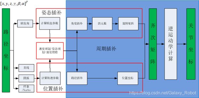
这里显示了速度规划化等和插补算法间的关系，这里不打算研究速度规划，因此姿态插补和位置补中，直接用了等距的步长。

首先用户输入姿态坐标一般是用欧拉角表示，即
$$p=[x,y,z,\gamma ,\beta ,\alpha {]}^T$$
因此需要把欧拉角转化为旋转矩阵。

假设用户输入的起点和终点位姿对应的旋转矩阵分别为$R_s,R_e$,设这两个姿态的旋转变换矩阵为$R$，则有
$$R_{s}R=R_e$$
注意这里是对矢量进行旋转，因此是右乘。因此旋转变换矩阵为
$$R=R_s^{-1}{R}_e$$
那么我们接下来实际是计算R的对应的欧拉参数，每次插补计算得到一个旋转矩阵$R_i$,机器人末端对应的姿态为$R_{si}=R_s{R}_i$ 。

姿态插补和位置插补均需要周期地循环计算，通过速度规划时就要保证姿态和位置的运动同步。

逆运动学计算的输入一般是齐次矩阵，输出是关节坐标。

下面仅针对直线路径的情形，把各个小模块写成C函数的形式，方便根据具体需求构建控制系统。

欧拉角转化为旋转矩阵

/**
* @brief 			Description: Algorithm for Computing the rotation matrix of the roll-pitch-yaw angles.
* @param[in]		roll			Angles for rotate around fix reference X axis.
* @param[in]		pitch			Angles for rotate around fix reference Y axis.
* @param[in]		yaw				Angles for rotate around fix reference Z axis.
* @param[out]		R				Rotation matrix.
* @return			No return value.
* @note:
*@warning:
*/
void RPYToRot(double roll, double pitch, double yaw, double R[3][3])
{
	double alpha = yaw;
	double beta = pitch;
	double gamma = roll;
	R[0][0] = cos(alpha)*cos(beta);
	R[0][1] = cos(alpha)*sin(beta)*sin(gamma) - sin(alpha)*cos(gamma);
	R[0][2] = cos(alpha)*sin(beta)*cos(gamma) + sin(alpha)*sin(gamma);
	R[1][0] = sin(alpha)*cos(beta);
	R[1][1] = sin(alpha)*sin(beta)*sin(gamma) + cos(alpha)*cos(gamma);
	R[1][2] = sin(alpha)*sin(beta)*cos(gamma) - cos(alpha)*sin(gamma);
	R[2][0] = -sin(beta);
	R[2][1] = cos(beta)*sin(gamma);
	R[2][2] = cos(beta)*cos(gamma);
	return;
}

姿态插补相关函数

	/**
	* @brief 			Description: structure of LinePath interpolation parameters.
	*/
	typedef struct
	{
		double p1[3];
		double p2[3];
		double L;
		double t[3];
		double pi[3];
		double Li;
		int InpFlag;
	}LineInpParam;


	/**
	* @brief 			Description: structure of arc interpolation parameters.
	*/
	typedef struct  
	{
		double p1[3];
		double p2[3];
		double p3[3];
		double N[3];
		double C[3];
		double theta;
		double R;
	}ArcInpParam;


	/**
	* @brief 			Description: structure of orientation interpolation parameters.
	*/
	typedef struct
	{
		double Rs[3][3];//Start orientation Rotation matrix. 
		double Re[3][3];//End orientation Rotation matrix.
		double R[3][3];	//Matrix rotation from Start orientation to End orientation.
		double omg[3];  //unit vector of Euler axis.
		double theta;	//Total interpolation angle.
		double Ri[3][3];//Current orientation rotation Matrix.
		double thetai;  //Current angle.
		int InpFlag;	//1:finish initial ,2;interpolating ,3;finish interpolation
	}OrientInpParam;


	/**
	* @brief 			Description: structure of line Path and Orientation (PO) interpolation parameters.
	*/
	typedef struct  
	{
		LineInpParam Line;
		OrientInpParam Orient;
		double Ts[4][4];
		double Te[4][4];
		double Ti[4][4];
		int InpFlag;
	}LinePOParam;

/**
 * @brief 			Description: Computes the parameters of  orientation interpolation between two orientations.
 * @param[in]		Rs				Start orientation.
 * @param[in]		Re				End orientation. 
 * @param[in]		Param			structure of orientation interpolation parameters..
 * @return			No return value.
 * @note:
 * @warning:
*/
void InitialOrientInpParam(double Rs[3][3],double Re[3][3], OrientInpParam *Param)
{
	double InvR[3][3];
	MatrixCopy((double *)Rs, 3, 3, (double *)Param->Rs);
	MatrixCopy((double *)Re, 3, 3, (double *)Param->Re);
	RotInv(Rs, InvR);
	MatrixMult((double *)InvR, 3, 3, (double *)Re, 3, (double *)Param->R);
	RotToAxisAng(Param->R, Param->omg, &Param->theta);
	MatrixCopy((double *)Param->R, 3, 3, (double *)Param->Ri);
	Param->thetai = 0.0;
	Param->InpFlag = 1;
	return;
}


/**
 * @brief 			Description: Computes orientations in each interpolation cycle.
 * @param[in]		Param			Interpolation parameter structure.
 * @param[out]		dtheta			angle  need to rotate from previous orientation to next orientation in next time step.
 * @return			Ri1				orientations in next interpolation cycle.
 * @retval			0
 * @note:
 * @warning:
*/
void QuaternionOrientInp(OrientInpParam *Param, double dtheta, double Ri1[3][3])
{
	double q[4];
	double R[3][3];
	Param->InpFlag = 2;
	Param->thetai = Param->thetai + dtheta;
	if (Param->thetai >= Param->theta)
	{
		Param->thetai = Param->theta;
		Param->InpFlag = 3;
	}
	AxisAngToQuaternion(Param->omg, Param->thetai, q);
	QuaternionToRot(q, R);
	MatrixMult((double *)Param->Rs, 3, 3, (double *)R, 3, (double *)Ri1);
	MatrixCopy((double *)Ri1, 3, 3, (double *)Param->Ri);
	return;
}

直线路径插补相关函数

/**
 * @brief 			Description:Computes the parameters of line path for interpolation.
 * @param[in]		p1				Coordinates of start point.
 * @param[in]		p2				Coordinates of end point.
 * @param[out]		p				Line path parameters structure.
 * @return			No return value.
 * @note:
 * @warning:
*/
void InitialLinePathParam(double p1[3],double p2[3], LineInpParam *p)
{
	int i;
	for (i=0;i<3;i++)
	{
		p->p1[i] = p1[i];
		p->p2[i] = p2[i];
		p->pi[i] = p1[i];
	}
	p->L = sqrt((p2[0] - p1[0])*(p2[0] - p1[0]) + (p2[1] - p1[1])*(p2[1] - p1[1]) + (p2[2] - p1[2])*(p2[2] - p1[2]));

	if (p->L<ZERO_DISTANCE)
	{
		p->t[0] = 0.0;
		p->t[1] = 0.0;
		p->t[2] = 0.0;
	}
	else
	{ 
		p->t[0] = (p2[0] - p1[0]) / p->L;
		p->t[1] = (p2[1] - p1[1]) / p->L;
		p->t[2] = (p2[2] - p1[2]) / p->L;
	}
	p->InpFlag = 1;
	p->Li = 0;
	return;
}

/**
 * @brief 			Description:Computes the line path interpolation coordinates in each interpolation cycle.
 * @param[in]		p				Line path parameters structure.
 * @param[in]		dL				step length in next interpolation cycle. 
 * @param[in]		pi1				coordinates in next interpolation cycle.
 * @return			No return value.
 * @note:
 * @warning:
*/
void LinePathInp(LineInpParam *p, double dL, double pi1[3])
{
	p->InpFlag = 2;
	if (p->Li + dL>=p->L)
	{
		pi1[0] = p->p2[0];
		pi1[1] = p->p2[1];
		pi1[2] = p->p2[2];
		p->Li = p->L;
		p->InpFlag = 3;
	}
	else if ( p->L- p->Li < 2.0*dL)
	{
		//avoid distance of  final step  is too small.
		dL = 0.5*dL;
		pi1[0] = p->pi[0] + p->t[0] * dL;
		pi1[1] = p->pi[1] + p->t[1] * dL;
		pi1[2] = p->pi[2] + p->t[2] * dL;
		p->Li = p->Li+dL;
	}
	else
	{
		pi1[0] = p->pi[0] + p->t[0] * dL;
		pi1[1] = p->pi[1] + p->t[1] * dL;
		pi1[2] = p->pi[2] + p->t[2] * dL;
		p->Li = p->Li + dL;
	}

	p->pi[0] = pi1[0];
	p->pi[1] = pi1[1];
	p->pi[2] = pi1[2];
	return;
}

把姿态插补和直线路径插补封装在一起，得到直线的位姿插补函数

/**
 * @brief 			Description: Computes the parameters of both line path and orientation for interpolation.
 * @param[in]		p1				Start coordinates,including x,y,z coordinates and orientation angles roll-pitch-yaw angles.
 * @param[in]		p2				End coordinates,including x,y,z coordinates and orientation angles roll-pitch-yaw angles.
 * @param[out]		LPO				Parameters of both line path and orientation for interpolation.
 * @return			No return value.
 * @note:
 * @warning:
*/
void InitialLinePOInpParam( double p1[6], double p2[6], LinePOParam *LPO)
{
	double Rs[3][3];
	double Re[3][3];
	RPYToRot(p1[3], p1[4], p1[5], Rs);
	RPYToRot(p2[3], p2[4], p2[5], Re);
	InitialLinePathParam( p1, p2, &(LPO->Line));
	InitialOrientInpParam(Rs, Re, &(LPO->Orient));
	RpToTrans(Rs, p1, LPO->Ts);
	RpToTrans(Rs, p1, LPO->Ti);
	RpToTrans(Re, p2, LPO->Te);
	LPO->InpFlag = 1;
	return;
}

/**
 * @brief 			Description:Computes the line path interpolation coordinates and orientation in each interpolation cycle.
 * @param[out]		LPO				Line path and orientation parameters structure.
 * @param[in]		dL				Line path interpolation step length.
 * @param[out]		dtheta			angle interpolation step length for Orientation interpolation.
 * @return			No return value.
 * @note:
 * @warning:
*/
void LinePOInp(LinePOParam *LPO,double dL,double dtheta,double Ti[4][4])
{
	double pi[3];
	double Ri[3][3];
	LPO->InpFlag = 2;
	LinePathInp(&LPO->Line, dL, pi);
	QuaternionOrientInp(&LPO->Orient, dtheta, Ri);
	if (LPO->Line.InpFlag==3 && LPO->Orient.InpFlag==3)
	{
		LPO->InpFlag = 3;
	}
	RpToTrans(Ri, pi, Ti);
	MatrixCopy((double *)Ti, 4, 4, (double *)LPO->Ti);
	return;
}

仿真验证

有了上面的函数，以及前面博客机器人学之逆运动学数值解法及SVD算法的逆运动学计算等模块，我们就可以集成一个直线路径的位姿插补程序。

（1）下面以UR3机器人为例，我们对两条线段进行插补，路径的坐标为

p1[6] = { 213.0,267.8,478.95,0,0,0 };

p2[6] = { 10,425,200, -PI / 2,0 ,0 };

p2[6] = { -10,525,200,-PI / 4,0,-PI / 6 };

插补生成路径的位置和姿态序列，进行逆运动学计算，得到关节坐标序列。仿真结果如下(动画是循环播放，实际路径是两条线段)。

示例程序如下

void test_LinePOInp()
{
	double p1[6] = { 213.0,267.8,478.95,0,0,0 };
	double p2[6] = { 10,425,200, -PI / 2,0 ,0 };
	//double p1[6] = { 10,425,200, -PI / 2,0 ,0 };
	//double p2[6] = { -10,525,200,-PI / 4,0,-PI / 6 };
	double Ti[4][4];
	double dL = 1;
	FILE *fp1;
	int ret = fopen_s(&fp1, "LineTrajactory.txt","w");
	if (ret)
	{
		printf("fopen_s error %d\n", ret);
	}
	LinePOParam pt;
	InitialLinePOInpParam(p1, p2, &pt);
	double dtheta = pt.Orient.theta/(pt.Line.L / dL);
	int JointNum = 6;
	double Slist[6][6] = {
		0 ,        0,         0,         0 ,        0,         0,
		0 ,   1.0000 ,   1.0000 ,   1.0000,         0,    1.0000,
		1.0000,         0 ,        0 ,        0 ,   1.0000,         0,
		0, -151.9000, -395.5500, -395.5500 , 110.4000 ,-478.9500,
		0 ,        0 ,        0  ,       0 ,-213.0000,         0,
		0  ,       0 ,        0,  213.0000 ,        0,  213.0000
	};
	double M[4][4] =
	{
		1.0000 ,        0,         0,  213.0000,
		0 ,   1.0000 ,        0,  267.8000,
		0 ,        0 ,   1.0000,  478.9500,
		0 ,        0  ,       0,    1.0000,
	};
	double thetalist0[6] = { 0 };
	//double thetalist0[6] = { 1.284569 ,0.488521, - 0.443200, 1.525477, - 1.570797, - 0.286227 };

	double thetalist[6];
	double eomg = 0.001;
	double ev = 0.01;
	while (pt.InpFlag!=3)
	{
		LinePOInp(&pt, dL, dtheta, Ti);
		IKinSpaceNR(JointNum,(double *)Slist, M, Ti, thetalist0,eomg,ev,10,thetalist);
		//MatrixCopy((double *)Ti, 4, 4, (double *)M);
		MatrixCopy(thetalist, 6, 1, thetalist0);//当前关节坐标作为下次逆解计算的初值.
        //把关节坐标写入文件
		fprintf(fp1, "%lf %lf %lf %lf %lf %lf\n", thetalist[0], thetalist[1], thetalist[2], thetalist[3], thetalist[4], thetalist[5]);
	}
	fclose(fp1);
	return;
}

（2）定点姿态插补

假设我们输入的两个坐标位置一样，只是姿态不同，那么应该能实现定点姿态插补。

p1[6] = { 10,425,200, -PI / 2,0 ,0 };
p2[6] = { 10,425,200, -PI *3/ 4,0 ,PI / 2 };

类似上面插补的示例程序，对两个路径做直线插补，计算的关节坐标进行仿真，效果如下图

示例程序如下

void test_LinePOInp()
{
	//double p1[6] = { 213.0,267.8,478.95,0,0,0 };
	//double p2[6] = { 10,425,200, -PI / 2,0 ,0 };
	//double p1[6] = { 10,425,200, -PI / 2,0 ,0 };
	//double p2[6] = { -10,525,200,-PI / 4,0,-PI / 6 };
	double p1[6] = { 10,425,200, -PI / 2,0 ,0 };
	double p2[6] = { 10,425,200, -PI *3/ 4,0 ,PI / 2 };
	double Ti[4][4];
	double dL = 1;
	FILE *fp1;
	int ret = fopen_s(&fp1, "LineTrajactory.txt","w");
	if (ret)
	{
		printf("fopen_s error %d\n", ret);
	}
	LinePOParam pt;
	InitialLinePOInpParam(p1, p2, &pt);
	//double dtheta =pt.Orient.theta/(pt.Line.L / dL);
	double dtheta = PI / 100;
	int JointNum = 6;
	double Slist[6][6] = {
		0 ,        0,         0,         0 ,        0,         0,
		0 ,   1.0000 ,   1.0000 ,   1.0000,         0,    1.0000,
		1.0000,         0 ,        0 ,        0 ,   1.0000,         0,
		0, -151.9000, -395.5500, -395.5500 , 110.4000 ,-478.9500,
		0 ,        0 ,        0  ,       0 ,-213.0000,         0,
		0  ,       0 ,        0,  213.0000 ,        0,  213.0000
	};
	double M[4][4] =
	{
		1.0000 ,        0,         0,  213.0000,
		0 ,   1.0000 ,        0,  267.8000,
		0 ,        0 ,   1.0000,  478.9500,
		0 ,        0  ,       0,    1.0000,
	};
	//double thetalist0[6] = { 0 };
	double thetalist0[6] = { 1.284569 ,0.488521, - 0.443200, 1.525477, - 1.570797, - 0.286227 };

	double thetalist[6];
	double eomg = 0.001;
	double ev = 0.01;
	while (pt.InpFlag!=3)
	{
		LinePOInp(&pt, dL, dtheta, Ti);
		IKinSpaceNR(JointNum,(double *)Slist, M, Ti, thetalist0,eomg,ev,10,thetalist);
		//MatrixCopy((double *)Ti, 4, 4, (double *)M);
		MatrixCopy(thetalist, 6, 1, thetalist0);
		fprintf(fp1, "%lf %lf %lf %lf %lf %lf\n", thetalist[0], thetalist[1], thetalist[2], thetalist[3], thetalist[4], thetalist[5]);
	}
	fclose(fp1);
	return;
}

逆解的关节坐标序列如下

1.289932 0.496461 -0.458281 1.540103 -1.584799 -0.307921
1.295334 0.504302 -0.472991 1.554231 -1.598923 -0.329481
1.300770 0.512033 -0.487316 1.567856 -1.613161 -0.350925
1.306238 0.519643 -0.501232 1.580967 -1.627510 -0.372268
1.311735 0.527116 -0.514715 1.593553 -1.641965 -0.393525
1.317257 0.534438 -0.527739 1.605603 -1.656523 -0.414710
1.322802 0.541595 -0.540278 1.617102 -1.671178 -0.435840
1.328368 0.548571 -0.552304 1.628036 -1.685928 -0.456928
1.333951 0.555352 -0.563789 1.638391 -1.700769 -0.477991
1.339549 0.561922 -0.574706 1.648150 -1.715695 -0.499044
1.345159 0.568267 -0.585024 1.657297 -1.730704 -0.520101
1.350778 0.574370 -0.594715 1.665811 -1.745792 -0.541180
1.356404 0.580217 -0.603749 1.673676 -1.760954 -0.562295
1.362033 0.585792 -0.612097 1.680872 -1.776185 -0.583462
1.367662 0.591081 -0.619729 1.687377 -1.791483 -0.604697
1.373289 0.596069 -0.626617 1.693172 -1.806842 -0.626016
1.378910 0.600741 -0.632733 1.698236 -1.822257 -0.647437
1.384522 0.605086 -0.638051 1.702547 -1.837724 -0.668974
1.390121 0.609089 -0.642543 1.706084 -1.853237 -0.690645
1.395705 0.612740 -0.646188 1.708826 -1.868790 -0.712467
1.401271 0.616028 -0.648963 1.710753 -1.884378 -0.734457
1.406813 0.618943 -0.650849 1.711842 -1.899994 -0.756633
1.412329 0.621477 -0.651829 1.712076 -1.915631 -0.779012
1.417815 0.623625 -0.651889 1.711433 -1.931281 -0.801613
1.423267 0.625381 -0.651018 1.709895 -1.946939 -0.824454
1.428681 0.626741 -0.649208 1.707445 -1.962594 -0.847553
1.434053 0.627706 -0.646456 1.704065 -1.978238 -0.870930
1.439378 0.628275 -0.642761 1.699741 -1.993862 -0.894604
1.444653 0.628450 -0.638125 1.694456 -2.009455 -0.918595
1.449873 0.628237 -0.632555 1.688197 -2.025008 -0.942922
1.455034 0.627642 -0.626062 1.680950 -2.040508 -0.967606
1.460131 0.626672 -0.618659 1.672705 -2.055945 -0.992667
1.465159 0.625339 -0.610363 1.663451 -2.071304 -1.018126
1.470113 0.623654 -0.601196 1.653176 -2.086573 -1.044004
1.474990 0.621632 -0.591179 1.641872 -2.101738 -1.070322
1.479784 0.619287 -0.580340 1.629531 -2.116783 -1.097101
1.484490 0.616636 -0.568707 1.616144 -2.131693 -1.124362
1.489104 0.613699 -0.556313 1.601706 -2.146451 -1.152127
1.493620 0.610496 -0.543190 1.586210 -2.161040 -1.180417
1.498035 0.607047 -0.529374 1.569651 -2.175441 -1.209252
1.502342 0.603376 -0.514903 1.552024 -2.189637 -1.238653
1.506538 0.599505 -0.499817 1.533327 -2.203606 -1.268639
1.510617 0.595461 -0.484156 1.513557 -2.217329 -1.299229
1.514576 0.591268 -0.467963 1.492712 -2.230784 -1.330442
1.518409 0.586954 -0.451280 1.470795 -2.243950 -1.362294
1.522112 0.582544 -0.434153 1.447806 -2.256802 -1.394800
1.525680 0.578068 -0.416627 1.423751 -2.269320 -1.427975
1.529110 0.573553 -0.398748 1.398637 -2.281477 -1.461829
1.532398 0.569028 -0.380564 1.372472 -2.293250 -1.496373
1.535539 0.564522 -0.362122 1.345270 -2.304615 -1.531613
1.538529 0.560062 -0.343471 1.317049 -2.315546 -1.567553
1.541366 0.555678 -0.324660 1.287827 -2.326017 -1.604192
1.544046 0.551397 -0.305737 1.257632 -2.336004 -1.641529
1.544046 0.551397 -0.305737 1.257632 -2.336004 -1.641529
1.544046 0.551397 -0.305737 1.257632 -2.336004 -1.641529

小结

在学习过程中，我对机器人算法的程序不断更新迭代，完整程序在gihub可下载-链接

经过本文的研究，对机械臂的姿态插补实现基本掌握了。两个姿态间插补算法可以总结为以下几步

（1）把输入起点和终点欧拉角转换为旋转矩阵$R_s,R_e$。

（2）两个姿态间的变换矩阵$R=R_s^{-1}{R}_e$。

（3）由旋转矩阵R计算等效轴和转角(即欧拉参数)，并写出对应的四元数。

（4）四元数转化为旋转矩阵$R_i$,计算中间姿态序列$R_{si}=R_s{R}_i$ .

（5）综合姿态和位置，得到表示位姿的齐次矩阵序列$T_{si}$。

---

参考文献

[1] Kenvin M. Lynch , Frank C. Park, Modern Robotics Mechanics,Planning , and Control[M]. May 3, 2017

[2]季晨. 工业机器人姿态规划及轨迹优化研究[D]. 哈尔滨工业大学, 2013.

[3] 程国采.四元数法及其应用[M].湖南：国防科技大学出版社，1991.