- 数字图像处理(一系列对图像进行处理、分析和改进的技术)
编程日记✧
智能医疗计算机视觉图像处理人工智能
数字图像处理是指对图像进行一系列的数学和算法处理,以增强、分析或理解图像的内容。这些处理包括从基础的像素操作到复杂的高维变换和机器学习模型。1.图像降噪在图像获取和传输过程中,往往会引入噪声。降噪技术用于减少这些噪声,同时尽量保持图像的细节。常见方法有:均值滤波:将像素邻域内的像素值取平均值,从而平滑图像。这种方法简单但可能会模糊边缘。高斯滤波:使用高斯函数为权重对像素进行加权平均,可以更好地平滑
- 基于语言的三种图像简单去噪算法:高效C++实现
m0_57781768
C语言(C++)算法研究和解读算法c++计算机视觉
基于语言的三种图像简单去噪算法:高效C++实现图像处理在现代计算机视觉中占有重要地位,而去噪处理则是图像处理的重要环节之一。本文将介绍三种基于语言的简单图像去噪算法,并提供详细的C++实现。我们将重点介绍均值滤波、中值滤波和高斯滤波三种方法,并探讨它们在图像去噪中的应用和效果。引言在数字图像处理中,噪声是不可避免的。它可能是由传感器噪声、传输错误或压缩伪影引起的。去噪的目的是在保留图像重要特征的同
- 24.7.27学习笔记
kkkkk021106
学习笔记
(按照老师发的学习计划走)先学习数字图像处理:1.单色图像0-255黑到白2.彩色图像:红绿蓝三元组的二维矩阵0-255像元(Pixel,图像元素的简称)是数字图像中最小的单元,代表图像中的一个点。每个像元都有一个特定的颜色和亮度值,组合在一起形成完整的图像。以下是关于像元的一些关键点:定义:像元是构成数字图像的基本单元。每个像元通常由多个颜色通道(如红色、绿色和蓝色)组成每个像元的颜色通常用数字
- 数字图像处理 - 形态学腐蚀
HelloZEX
数字图像处理C++图像处理opencv形态学处理
一、理论与概念讲解——从现象到本质1.1形态学概述形态学(morphology)一词通常表示生物学的一个分支,该分支主要研究动植物的形态和结构。而我们图像处理中指的形态学,往往表示的是数学形态学。下面一起来了解数学形态学的概念。数学形态学(Mathematicalmorphology)是一门建立在格论和拓扑学基础之上的图像分析学科,是数学形态学图像处理的基本理论。其基本的运算包括:二值腐蚀和膨胀、
- matlab计算正交变换,图像的正交变换matlab.pdf
大Victor
matlab计算正交变换
图像的正交变换matlab《数字图像处理》课程实验报告实验名:图像的正交变换实验1院系:自动化测试与控制系班级:1201132姓名:李丹阳学号:1120110113哈尔滨工业大学电气工程及自动化学院光电信息工程2015年12月13日一、实验原理二、实验内容三、实验结果与分析1、傅立叶变换A)绘制一个二值图像矩阵,并将其傅立叶函数可视化。(傅里叶变换A)的实验结果B)利用傅立叶变换分析两幅图像的相关
- MATLAB--数字图像处理 图像几何变换
海轰Pro
一、实验名称图像的几何变换二、实验目的1.熟悉MATLAB软件的使用。2.掌握图像几何变换的原理及数学运算。3.于MATLAB环境下编程实现对图片不同的几何变换。三、实验内容1.将图像绕图像中心顺时针旋转30度,旋转之后的图像尺寸保持为原图像的尺寸。2.将原图像放大2倍3.得到该图像的水平镜像图片4.得到该图像的垂直错切图像四、实验仪器与设备Win1064位电脑MATLAB2017a五、实验原理图
- 《数字图像处理-OpenCV/Python》连载:形态学图像处理
youcans_
opencvpython图像处理计算机视觉人工智能
《数字图像处理-OpenCV/Python》连载:形态学图像处理本书京东优惠购书链接https://item.jd.com/14098452.html本书CSDN独家连载专栏https://blog.csdn.net/youcans/category_12418787.html第12章形态学图像处理形态学图像处理是基于形状的图像处理,基本思想是利用各种形状的结构元进行形态学运算,从图像中提取表达和
- 数字图像处理2——图像基本运算
苏俗
数字图像处理实战opencv人工智能计算机视觉
1.改写彩色图像像素的RGB值#RGB真彩色图像的数据结构#导入用到的包importnumpyasnpimportcv2ascvimportmatplotlib.pyplotasplt%matplotlibinline#读入一幅彩色图像img=cv.imread('./imagedata/old_villa.jpg',cv.IMREAD_COLOR)img2=img.copy()print('数组
- 如何用 Canvas 实现 PS 的液化功能
最近在做业务需求时,需要实现对图片的液化功能,类似于美图秀秀的瘦脸功能。这已经不仅是图片缩放、拖动、剪裁这类对图片整体的操作了,而是需要对图片的像素进行一系列的计算和修改,那么该怎么实现这个功能呢?基础知识在进入正题之前,我们先来了解一些数字图像处理和Canvas的基础知识。图像处理里的像素是什么现实世界中,人眼直接看到的图像或者在相机中拍摄到的影像,这类图片的最大特点是图像相关的物理量变化是连续
- 视频剪辑,人脸贴纸美颜特效数字图像处理背后的技术-Qt版本
chenchao_shenzhen
Qt音视频开发计算机视觉qt5音视频数字图像处理视频剪辑人脸特效
Qt能做什么?其实大部分都是一些c++最擅长的领域,客户端软件,工具软件。Qt最擅长什么?这个看主流的行业巨头,比如Autodesk的3D建模动画软件maya,Adobe的3D贴图绘制软件SubstancePainter,音视频剪辑软件三巨头之一达芬奇。这三家都是行业垄断巨头之一,所以2010年之后,我们说Qt开发过什么软件,就不能只说vlc,googleEarth了。甚至你跑到开源社区去看,80
- 矩阵与计算机论文,数字图像处理中矩阵变换的应用探索-数字图像处理论文-计算机论文.docx...
weixin_39977642
矩阵与计算机论文
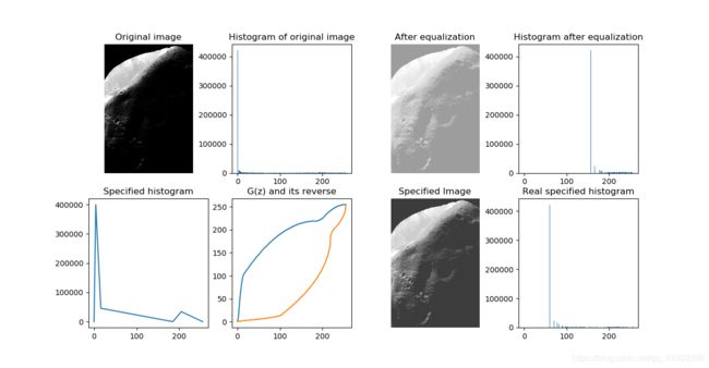
数字图像处理中矩阵变换的应用探索-数字图像处理论文-计算机论文——文章均为WORD文档,下载后可直接编辑使用亦可打印——摘要:从矩阵变换入手,将矩阵变换应用到图像处理中,且通过直方图匹配法及欧几里得距离法求取相似度来进行人脸识别和预测。所得实验结果直观高效,相似度均能达到90%以上。关键词:数字图像处理;矩阵变换;人脸识别和预测;相似度;Abstract:Thispaperstartswithma
- 矩阵在计算机图像处理中的应用,英语翻译在实际应用中,矩阵不仅对于我们求解线性方程组提供了很好的方法,还在计算机等领域得到了广泛的应用:数字图像处理,人...
光露
矩阵在计算机图像处理中的应用
共回答了21个问题采纳率:100%Inpracticalapplication,thematrisisnotonlyprovideagoodmethodforustosolvelinearsimultaneousequations,butalsoputintowidelyuseincomputerfield:digitalimageprosessing,ArtificialIntelligence
- Python中使用opencv-python进行人脸检测
雪域迷影
OpenCVPython编程编程语言学习opencvpython人工智能
Python中使用opencv-python进行人脸检测之前写过一篇VC++中使用OpenCV进行人脸检测的博客。以数字图像处理中经常使用的lena图像为例,如下图所示:使用OpenCV进行人脸检测十分简单,OpenCV官网给了一个Python人脸检测的示例程序,objectDetection.py代码如下:from__future__importprint_functionimportcv2as
- OpenCV入门:图像处理的基石
白猫a~
编程opencv
在数字图像处理领域,OpenCV(开源计算机视觉库)是一个不可或缺的工具。它包含了一系列强大的算法和函数,使得开发者可以轻松地处理图像和视频数据。本文将带你走进OpenCV的世界,了解其基本概念和常见应用。1.OpenCV简介OpenCV,全称OpenSourceComputerVisionLibrary,是一个开源的计算机视觉和机器学习库。它支持多种编程语言,包括C++、Python、Java等
- 如何用 Canvas 实现 PS 的液化功能
最近在做业务需求时,需要实现对图片的液化功能,类似于美图秀秀的瘦脸功能。这已经不仅是图片缩放、拖动、剪裁这类对图片整体的操作了,而是需要对图片的像素进行一系列的计算和修改,那么该怎么实现这个功能呢?基础知识在进入正题之前,我们先来了解一些数字图像处理和Canvas的基础知识。图像处理里的像素是什么现实世界中,人眼直接看到的图像或者在相机中拍摄到的影像,这类图片的最大特点是图像相关的物理量变化是连续
- 【全网最低价】司守奎《数学建模算法与应用》第三版pdf+数学建模资料(非常详细的算法学习和路线)小白推荐
阿贵学长
数学建模学习算法matlab性能优化深度学习
1.《数学建模算法与应用》主要内容包括时间序列、支持向量机、偏最小二乘面归分析、现代优化算法、数字图像处理、综合评价与决策方法、预测方法以及数学建模经典算法等内容。文章末尾有电子版PDF文件链接2.算法学习流程及详细过程主要算法:工具箱推荐遗传算法-beatxbx工具箱,求解速度很快,并行计算LIBSVM-比MATLAB自带工具箱好用得多yamlip,特别推荐,统一优化求解工具箱由于文件很多,学长
- 数字图像处理与Python语言实现-常见图像特效(一)
视觉&物联智能
数字图像处理与Python实现python开发语言数字图像处理图像处理人工智能机器视觉计算机视觉
文章目录0、准备1、亮度调节2、细节强化3、底片效果4、卡通效果5、浮雕效果6、铅笔素描效果7、夏季或温色滤镜8、冬季或冷色滤波在本文中将演示使用OpenCV来模仿流行的Photoshop或Instagram滤镜的各种图像处理技术。在文章中,我们将尝试使用各种滤镜,其中许多滤镜会生成原始图像的艺术效果图。正如您将在文章中看到的,其中许多效果需要进行一些实验,并且给定滤镜的结果可能会根据所使用的特定
- 数字图像处理与Python语言实现-常见图像特效(三)
视觉&物联智能
数字图像处理与Python实现python计算机视觉opencv人工智能图像处理机器视觉图像特效
文章目录18、提高曝光度19、轮廓滤镜/图像锐化20、风格化滤镜21、颜色化滤镜22、扩散/毛玻璃效果23、碧绿效果24、漫画效果25、边缘发光/增强效果26、冰冻效果本文为前面文章:数字图像处理与Python语言实现-常见图像特效(二)数字图像处理与Python语言实现-常见图像特效(一)的延续。18、提高曝光度def
- CT重建 平行射线滤波反投影
73826669
图像处理傅立叶分析图像处理
计算机断层重建(CT)是一个比较热门的领域,这篇文章简单介绍了反投影方法的重建过程。参考资料:冈萨雷斯,《数字图像处理》,电子工业出版社。文章目录直接反投影投影与Radon变换滤波反投影法(FBP)傅里叶切片定理平行射线下的滤波反投影重建卷积与傅里叶反变换直接反投影该方法是沿着射线来的方向把一维信号反投影回去,可以想象成把投影穿过图像区域反“涂抹”回去。注意到相隔180°的投影互为镜像,因此,为了
- 数字图像处理实验记录七(彩色图像处理实验)
泉绮
数字图像处理实验记录计算机视觉图像处理opencv
一、基础知识经过前面的实验可以得知,彩色图像中的RGB图像就是一个三维矩阵,有3个维度,它们分别存储着R元素,G元素,B元素的灰度信息,最后将它们合起来,便是彩色图像。这一次实验涉及CMYK和HSI颜色模型,不妨搜索一下:CMYK:CMYK颜色模型包括青(cyan)、品红(magenta)、黄(yellow)和黑(black),为避免与Blue混淆,黑色用K表示。彩色打印、印刷等应用领域采用打印墨
- 形态学操作之开操作与闭操作的python实现——数字图像处理
筱筱西雨
图像处理python计算机视觉人工智能图像处理算法
原理图像处理中的开操作(Opening)和闭操作(Closing)是形态学(Morphological)操作的两个基本类型,它们都是基于膨胀(Dilation)和腐蚀(Erosion)操作。这些操作通常用于二值化图像,但也可以应用于灰度图像。腐蚀(Erosion)腐蚀操作的目的是缩小或消除图像中的前景(通常是白色)对象。在腐蚀操作中,使用一个结构元素(或核)在图像上滑动。如果结构元素在某个位置下的
- 数字图像处理实验记录十(图像分割实验)
泉绮
数字图像处理实验记录计算机视觉图像处理opencv
一、基础知识1、什么是图像分割图像分割就是指把图像分成各具特性的区域并提取出感兴趣目标的技术和过程,特性可以是灰度、颜色、纹理等,目标可以对应单个区域,也可以对应多个区域。2、图像分割是怎么实现的图像分割算法基于像素值的不连续性和相似性,不连续性是图像的边缘,再根据制定的准则将图像分割为相似的区域,如阈值处理、区域生长、区域分离和聚合。二、实验要求三、实验记录(具体任务只展示对图片1的处理)总代码
- 数字图像处理实验记录八(图像压缩实验)
泉绮
数字图像处理实验记录图像处理matlab
前言:做这个实验的时候很忙,就都是你抄我我抄你了一、基础知识1.为什么要进行图像压缩:图像的数据量巨大,对计算机的处理速度、存储容量要求高。传输信道带宽、通信链路容量一定,需要减少传输数据量,提高通信速度。因此要进行图像压缩,减少数据量。2.怎么进行图像压缩:我们使用霍夫曼编码进行压缩。霍夫曼编码原理是利用信息符号概率分布特性的变字长的编码方法。对于出现概率大的信息符号编以短字长的码,对于出现概率
- 数字图像处理实验记录九(数字形态学实验)
泉绮
数字图像处理实验记录计算机视觉图像处理matlab
一、基础知识1.形态学,用于从图像中提取对表达和描绘区域形状有意义的图像分量,使后续的识别工作能够抓住目标对象最为有本质的形状特征,如边界连通区域等。2.膨胀运算:膨胀会使目标区域范围“变大”,将于目标区域接触的背景点合并到该目标物中,使目标边界向外部扩张。作用就是可以用来填补目标区域中某些空洞以及消除包含在目标区域中的小颗粒噪声。3.腐蚀运算:腐蚀可以使目标区域范围“变小”,其实质造成图像的边界
- 关于数字图像处理考试
泉绮
数字图像处理实验记录计算机视觉opencv图像处理
我们学校这门科目是半学期就完结哦,同学们学习的时候要注意时间哦。选择题不用管,到时候会有各种版本的复习资料的。以下这些东西可能会是大题的重点:我根据平时代码总结的,供参考基本操作:1.读图:imread(‘图片路径’)2.显示图:imshow(图片)3.开新窗口:figure()4.rgb转灰度图:rgb2gray(图片)5.灰度图合成彩色图:图片=cat(3,灰度图1,灰度图2,灰度图3);实验
- re:从0开始的CSS学习之路 5. 颜色单位
扶摇|
从0开始的CSS之旅css学习前端
0.写在前面没想到在CSS里也要再次了解这些颜色单位,感觉回到了大二的数字图像处理,可惜现在已经大四了,感觉并没有学会什么AI的东西1.颜色单位预定义颜色名:HTML和CSS规定了147种颜色名。例如:redyellowgreenblueRGB颜色值rgb(red,green,blue):括号中每个参数代表对应颜色的浓度浓度值是0-255之间的整数,0表示无浓度,255表示最大浓度也可以使用百分比
- 数字图像处理与Python语言实现-常见图像特效(二)
视觉&物联智能
数字图像处理与Python实现pythonopencv计算机视觉人工智能图像处理机器视觉图像特效
文章目录9、Splash滤镜10、双色调(Duo-Tone)滤镜11、日光(Daylight)滤镜12、60sTVs效果13、高对比度14、棕褐色/复古滤镜15、晕影效果16、模糊滤镜17、浮雕边缘9、Splash滤镜在Splash滤镜中,仅某些颜色保持原样,其余颜色转换为灰度。为了执行此操作,我们将在HSV颜色空间中使用cv2.inRange。这可用于形成具有该范围内的值的所有像素的掩码,并且这
- 数字图像处理(实践篇)四十三 OpenCV-Python 使用SURF算法检测图像上的特征点的实践
Jackilina_Stone
数字图像处理(入门篇实践篇综合篇)python数字图像处理计算机视觉OpenCV
目录一SURF算法概述1积分图2SURF算法3SIFT与SURF二涉及的函数三实践一SURF算法概述
- 【数字图像处理】2021期末复习考试重点大纲
Rose J
复习数组图像处理复习
本文目录数字图像处理期末复习1.填空(每空2分,共20分)1.均值滤波计算2.中值滤波计算3.水平方向一阶锐化计算4.无方向一阶锐化计算5.位图文件存储所需要的数据量计算2.问答(每题10分,共10分)1、什么是采样,简述采样间隔与图像的关系。2、什么是量化,简述量化等级与图像关系。3、简述中值滤波器对不同类型的噪声抑制效果。4、对于一张灰度图像,其梯度是如何定义的?图像梯度的物理意义是什么?3.
- 数字图像处理之二维码图像提取算法(十)
Snail_Walker
VideoCoding&ImageProopencv2threshold二值化
这里来说明一下做这次的二维码提取算法用到的函数,最后再给出完整的代码!进行图像的二值化,这里可以使用opencv2里的函数threshold,当然在opencv里也有cvThreshold函数(这个函数可以具体参考:http://blog.csdn.net/xuehuic/article/details/7401181)首先我们要了解:最简单的图像分割的方法。应用举例:从一副图像中利用阈值分割出我
- Java开发中,spring mvc 的线程怎么调用?
小麦麦子
springmvc
今天逛知乎,看到最近很多人都在问spring mvc 的线程http://www.maiziedu.com/course/java/ 的启动问题,觉得挺有意思的,那哥们儿问的也听仔细,下面的回答也很详尽,分享出来,希望遇对遇到类似问题的Java开发程序猿有所帮助。
问题:
在用spring mvc架构的网站上,设一线程在虚拟机启动时运行,线程里有一全局
- maven依赖范围
bitcarter
maven
1.test 测试的时候才会依赖,编译和打包不依赖,如junit不被打包
2.compile 只有编译和打包时才会依赖
3.provided 编译和测试的时候依赖,打包不依赖,如:tomcat的一些公用jar包
4.runtime 运行时依赖,编译不依赖
5.默认compile
依赖范围compile是支持传递的,test不支持传递
1.传递的意思是项目A,引用
- Jaxb org.xml.sax.saxparseexception : premature end of file
darrenzhu
xmlprematureJAXB
如果在使用JAXB把xml文件unmarshal成vo(XSD自动生成的vo)时碰到如下错误:
org.xml.sax.saxparseexception : premature end of file
很有可能时你直接读取文件为inputstream,然后将inputstream作为构建unmarshal需要的source参数。InputSource inputSource = new In
- CSS Specificity
周凡杨
html权重Specificitycss
有时候对于页面元素设置了样式,可为什么页面的显示没有匹配上呢? because specificity
CSS 的选择符是有权重的,当不同的选择符的样式设置有冲突时,浏览器会采用权重高的选择符设置的样式。
规则:
HTML标签的权重是1
Class 的权重是10
Id 的权重是100
- java与servlet
g21121
servlet
servlet 搞java web开发的人一定不会陌生,而且大家还会时常用到它。
下面是java官方网站上对servlet的介绍: java官网对于servlet的解释 写道
Java Servlet Technology Overview Servlets are the Java platform technology of choice for extending and enha
- eclipse中安装maven插件
510888780
eclipsemaven
1.首先去官网下载 Maven:
http://www.apache.org/dyn/closer.cgi/maven/binaries/apache-maven-3.2.3-bin.tar.gz
下载完成之后将其解压,
我将解压后的文件夹:apache-maven-3.2.3,
并将它放在 D:\tools目录下,
即 maven 最终的路径是:D:\tools\apache-mave
- jpa@OneToOne关联关系
布衣凌宇
jpa
Nruser里的pruserid关联到Pruser的主键id,实现对一个表的增删改,另一个表的数据随之增删改。
Nruser实体类
//*****************************************************************
@Entity
@Table(name="nruser")
@DynamicInsert @Dynam
- 我的spring学习笔记11-Spring中关于声明式事务的配置
aijuans
spring事务配置
这两天学到事务管理这一块,结合到之前的terasoluna框架,觉得书本上讲的还是简单阿。我就把我从书本上学到的再结合实际的项目以及网上看到的一些内容,对声明式事务管理做个整理吧。我看得Spring in Action第二版中只提到了用TransactionProxyFactoryBean和<tx:advice/>,定义注释驱动这三种,我承认后两种的内容很好,很强大。但是实际的项目当中
- java 动态代理简单实现
antlove
javahandlerproxydynamicservice
dynamicproxy.service.HelloService
package dynamicproxy.service;
public interface HelloService {
public void sayHello();
}
dynamicproxy.service.impl.HelloServiceImpl
package dynamicp
- JDBC连接数据库
百合不是茶
JDBC编程JAVA操作oracle数据库
如果我们要想连接oracle公司的数据库,就要首先下载oralce公司的驱动程序,将这个驱动程序的jar包导入到我们工程中;
JDBC链接数据库的代码和固定写法;
1,加载oracle数据库的驱动;
&nb
- 单例模式中的多线程分析
bijian1013
javathread多线程java多线程
谈到单例模式,我们立马会想到饿汉式和懒汉式加载,所谓饿汉式就是在创建类时就创建好了实例,懒汉式在获取实例时才去创建实例,即延迟加载。
饿汉式:
package com.bijian.study;
public class Singleton {
private Singleton() {
}
// 注意这是private 只供内部调用
private static
- javascript读取和修改原型特别需要注意原型的读写不具有对等性
bijian1013
JavaScriptprototype
对于从原型对象继承而来的成员,其读和写具有内在的不对等性。比如有一个对象A,假设它的原型对象是B,B的原型对象是null。如果我们需要读取A对象的name属性值,那么JS会优先在A中查找,如果找到了name属性那么就返回;如果A中没有name属性,那么就到原型B中查找name,如果找到了就返回;如果原型B中也没有
- 【持久化框架MyBatis3六】MyBatis3集成第三方DataSource
bit1129
dataSource
MyBatis内置了数据源的支持,如:
<environments default="development">
<environment id="development">
<transactionManager type="JDBC" />
<data
- 我程序中用到的urldecode和base64decode,MD5
bitcarter
cMD5base64decodeurldecode
这里是base64decode和urldecode,Md5在附件中。因为我是在后台所以需要解码:
string Base64Decode(const char* Data,int DataByte,int& OutByte)
{
//解码表
const char DecodeTable[] =
{
0, 0, 0, 0, 0, 0
- 腾讯资深运维专家周小军:QQ与微信架构的惊天秘密
ronin47
社交领域一直是互联网创业的大热门,从PC到移动端,从OICQ、MSN到QQ。到了移动互联网时代,社交领域应用开始彻底爆发,直奔黄金期。腾讯在过去几年里,社交平台更是火到爆,QQ和微信坐拥几亿的粉丝,QQ空间和朋友圈各种刷屏,写心得,晒照片,秀视频,那么谁来为企鹅保驾护航呢?支撑QQ和微信海量数据背后的架构又有哪些惊天内幕呢?本期大讲堂的内容来自今年2月份ChinaUnix对腾讯社交网络运营服务中心
- java-69-旋转数组的最小元素。把一个数组最开始的若干个元素搬到数组的末尾,我们称之为数组的旋转。输入一个排好序的数组的一个旋转,输出旋转数组的最小元素
bylijinnan
java
public class MinOfShiftedArray {
/**
* Q69 旋转数组的最小元素
* 把一个数组最开始的若干个元素搬到数组的末尾,我们称之为数组的旋转。输入一个排好序的数组的一个旋转,输出旋转数组的最小元素。
* 例如数组{3, 4, 5, 1, 2}为{1, 2, 3, 4, 5}的一个旋转,该数组的最小值为1。
*/
publ
- 看博客,应该是有方向的
Cb123456
反省看博客
看博客,应该是有方向的:
我现在就复习以前的,在补补以前不会的,现在还不会的,同时完善完善项目,也看看别人的博客.
我刚突然想到的:
1.应该看计算机组成原理,数据结构,一些算法,还有关于android,java的。
2.对于我,也快大四了,看一些职业规划的,以及一些学习的经验,看看别人的工作总结的.
为什么要写
- [开源与商业]做开源项目的人生活上一定要朴素,尽量减少对官方和商业体系的依赖
comsci
开源项目
为什么这样说呢? 因为科学和技术的发展有时候需要一个平缓和长期的积累过程,但是行政和商业体系本身充满各种不稳定性和不确定性,如果你希望长期从事某个科研项目,但是却又必须依赖于某种行政和商业体系,那其中的过程必定充满各种风险。。。
所以,为避免这种不确定性风险,我
- 一个 sql优化 ([精华] 一个查询优化的分析调整全过程!很值得一看 )
cwqcwqmax9
sql
见 http://www.itpub.net/forum.php?mod=viewthread&tid=239011
Web翻页优化实例
提交时间: 2004-6-18 15:37:49 回复 发消息
环境:
Linux ve
- Hibernat and Ibatis
dashuaifu
Hibernateibatis
Hibernate VS iBATIS 简介 Hibernate 是当前最流行的O/R mapping框架,当前版本是3.05。它出身于sf.net,现在已经成为Jboss的一部分了 iBATIS 是另外一种优秀的O/R mapping框架,当前版本是2.0。目前属于apache的一个子项目了。 相对Hibernate“O/R”而言,iBATIS 是一种“Sql Mappi
- 备份MYSQL脚本
dcj3sjt126com
mysql
#!/bin/sh
# this shell to backup mysql
#
[email protected] (QQ:1413161683 DuChengJiu)
_dbDir=/var/lib/mysql/
_today=`date +%w`
_bakDir=/usr/backup/$_today
[ ! -d $_bakDir ] && mkdir -p
- iOS第三方开源库的吐槽和备忘
dcj3sjt126com
ios
转自
ibireme的博客 做iOS开发总会接触到一些第三方库,这里整理一下,做一些吐槽。 目前比较活跃的社区仍旧是Github,除此以外也有一些不错的库散落在Google Code、SourceForge等地方。由于Github社区太过主流,这里主要介绍一下Github里面流行的iOS库。 首先整理了一份
Github上排名靠
- html wlwmanifest.xml
eoems
htmlxml
所谓优化wp_head()就是把从wp_head中移除不需要元素,同时也可以加快速度。
步骤:
加入到function.php
remove_action('wp_head', 'wp_generator');
//wp-generator移除wordpress的版本号,本身blog的版本号没什么意义,但是如果让恶意玩家看到,可能会用官网公布的漏洞攻击blog
remov
- 浅谈Java定时器发展
hacksin
java并发timer定时器
java在jdk1.3中推出了定时器类Timer,而后在jdk1.5后由Dou Lea从新开发出了支持多线程的ScheduleThreadPoolExecutor,从后者的表现来看,可以考虑完全替代Timer了。
Timer与ScheduleThreadPoolExecutor对比:
1.
Timer始于jdk1.3,其原理是利用一个TimerTask数组当作队列
- 移动端页面侧边导航滑入效果
ini
jqueryWebhtml5cssjavascirpt
效果体验:http://hovertree.com/texiao/mobile/2.htm可以使用移动设备浏览器查看效果。效果使用到jquery-2.1.4.min.js,该版本的jQuery库是用于支持HTML5的浏览器上,不再兼容IE8以前的浏览器,现在移动端浏览器一般都支持HTML5,所以使用该jQuery没问题。HTML文件代码:
<!DOCTYPE html>
<h
- AspectJ+Javasist记录日志
kane_xie
aspectjjavasist
在项目中碰到这样一个需求,对一个服务类的每一个方法,在方法开始和结束的时候分别记录一条日志,内容包括方法名,参数名+参数值以及方法执行的时间。
@Override
public String get(String key) {
// long start = System.currentTimeMillis();
// System.out.println("Be
- redis学习笔记
MJC410621
redisNoSQL
1)nosql数据库主要由以下特点:非关系型的、分布式的、开源的、水平可扩展的。
1,处理超大量的数据
2,运行在便宜的PC服务器集群上,
3,击碎了性能瓶颈。
1)对数据高并发读写。
2)对海量数据的高效率存储和访问。
3)对数据的高扩展性和高可用性。
redis支持的类型:
Sring 类型
set name lijie
get name lijie
set na
- 使用redis实现分布式锁
qifeifei
在多节点的系统中,如何实现分布式锁机制,其中用redis来实现是很好的方法之一,我们先来看一下jedis包中,有个类名BinaryJedis,它有个方法如下:
public Long setnx(final byte[] key, final byte[] value) {
checkIsInMulti();
client.setnx(key, value);
ret
- BI并非万能,中层业务管理报表要另辟蹊径
张老师的菜
大数据BI商业智能信息化
BI是商业智能的缩写,是可以帮助企业做出明智的业务经营决策的工具,其数据来源于各个业务系统,如ERP、CRM、SCM、进销存、HER、OA等。
BI系统不同于传统的管理信息系统,他号称是一个整体应用的解决方案,是融入管理思想的强大系统:有着系统整体的设计思想,支持对所有
- 安装rvm后出现rvm not a function 或者ruby -v后提示没安装ruby的问题
wudixiaotie
function
1.在~/.bashrc最后加入
[[ -s "$HOME/.rvm/scripts/rvm" ]] && source "$HOME/.rvm/scripts/rvm"
2.重新启动terminal输入:
rvm use ruby-2.2.1 --default
把当前安装的ruby版本设为默