DrGraph原理示教 - OpenCV 4 功能 - 直方图

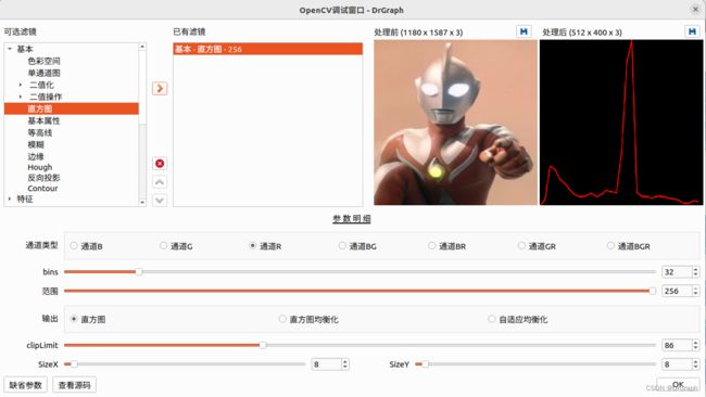
OpenCV直方图是一种可以对整幅图的灰度分布进行整体了解的图示。它是带有像素值（从0到255，不总是）的图在X轴上，在y轴上的图像对应的像素个数。通过观察图像的直方图，我们可以直观的了解图像的对比度、亮度、亮度分布等。
在直方图中，横坐标表示图像中各个像素点的灰度级，纵坐标表示具有该灰度级的像素个数。直方图的左边部分显示了图像中较暗像素的数量，右边区域显示了更明亮的像素。
直方图是非常常用的图像处理方法，有时在很多图像预处理中能起到特别好的效果。

一维直方图

OpenCV中，直方图是调用calxHist函数，该函数的参数比较多，不太好理解

The function cv::calcHist calculates the histogram of one or more arrays. The elements of a tuple used
to increment a histogram bin are taken from the corresponding input arrays at the same location. The
sample below shows how to compute a 2D Hue-Saturation histogram for a color image. :
@include snippets/imgproc_calcHist.cpp

@param images Source arrays. They all should have the same depth, CV_8U, CV_16U or CV_32F , and the same
size. Each of them can have an arbitrary number of channels.
@param nimages Number of source images.
@param channels List of the dims channels used to compute the histogram. The first array channels
are numerated from 0 to images[0].channels()-1 , the second array channels are counted from
images[0].channels() to images[0].channels() + images[1].channels()-1, and so on.
@param mask Optional mask. If the matrix is not empty, it must be an 8-bit array of the same size
as images[i] . The non-zero mask elements mark the array elements counted in the histogram.
@param hist Output histogram, which is a dense or sparse dims -dimensional array.
@param dims Histogram dimensionality that must be positive and not greater than CV_MAX_DIMS
(equal to 32 in the current OpenCV version).
@param histSize Array of histogram sizes in each dimension.
@param ranges Array of the dims arrays of the histogram bin boundaries in each dimension. When the
histogram is uniform ( uniform =true), then for each dimension i it is enough to specify the lower
(inclusive) boundary \f$L_0\f$ of the 0-th histogram bin and the upper (exclusive) boundary
\f$U_{\texttt{histSize}[i]-1}\f$ for the last histogram bin histSize[i]-1 . That is, in case of a
uniform histogram each of ranges[i] is an array of 2 elements. When the histogram is not uniform (
uniform=false ), then each of ranges[i] contains histSize[i]+1 elements:
\f$L_0, U_0=L_1, U_1=L_2, ..., U_{\texttt{histSize[i]}-2}=L_{\texttt{histSize[i]}-1}, U_{\texttt{histSize[i]}-1}\f$
. The array elements, that are not between \f$L_0\f$ and \f$U_{\texttt{histSize[i]}-1}\f$ , are not
counted in the histogram.
@param uniform Flag indicating whether the histogram is uniform or not (see above).
@param accumulate Accumulation flag. If it is set, the histogram is not cleared in the beginning
when it is allocated. This feature enables you to compute a single histogram from several sets of
arrays, or to update the histogram in time.
*/
CV_EXPORTS void calcHist( const Mat* images, int nimages,
                          const int* channels, InputArray mask,
                          OutputArray hist, int dims, const int* histSize,
                          const float** ranges, bool uniform = true, bool accumulate = false );

简单化理解，那就是hist参数之前的为输入参数，其余的为输出参数。
dims指定直方图的维数，可以先理解1维的。
因为calcHist函数可以用于多维，所以它的参数也要支持多维。其实嘛，简单点多好，多用几个函数分别实现相应多维，用得多的一二维直方图就用得轻松了。
正常使用，calcHist就针对一维处理。所以要用的时候，先需要将彩色图像灰度化，或者split取得各通首图像分别应用calcHist，然后相应算后再合并处理。如果只是想看直方图，那就直接画出来。

  		std::vector<Mat> mv;
   		split(dstMat, mv);  
        int histSize[] = { bins };
        float rgb_ranges[] = { 0, r };
        const float * ranges[] = { rgb_ranges };
        dstMat = CvHelper::ToMat_BGR(dstMat);
        int channels[] = { 0 };
        Mat b_hist, g_hist, r_hist;
        if(channelType == 0 || channelType == 3 || channelType == 4 || channelType == 6)    // B
            calcHist(&mv[0], 1, channels, Mat(), b_hist, 1, histSize, ranges, true, false);
        if(channelType == 1 || channelType == 3 || channelType == 5 || channelType == 6)    // G
            calcHist(&mv[1], 1, channels, Mat(), g_hist, 1, histSize, ranges, true, false);
        if(channelType == 2 || channelType == 4 || channelType == 5 || channelType == 6)    // R
            calcHist(&mv[2], 1, channels, Mat(), r_hist, 1, histSize, ranges, true, false);
        double maxVal = 0;
        int hist_w = 512;
        int hist_h = 400;
        int bin_w = cvRound((double)hist_w / histSize[0]);
        Mat histImage = Mat::zeros(hist_h, hist_w, CV_8UC3);
        normalize(b_hist, b_hist, 0, histImage.rows, NORM_MINMAX, -1, Mat());
        normalize(g_hist, g_hist, 0, histImage.rows, NORM_MINMAX, -1, Mat());
        normalize(r_hist, r_hist, 0, histImage.rows, NORM_MINMAX, -1, Mat());
        for(int i = 1; i < histSize[0]; ++i) {
            if(r_hist.empty() == false)
                line(histImage, Point(bin_w * (i - 1), hist_h - cvRound(r_hist.at<float>(i - 1))),
                     Point(bin_w * i, hist_h - cvRound(r_hist.at<float>(i))), Scalar(255, 0, 0), 2, LINE_AA, 0);
            if(g_hist.empty() == false)
                line(histImage, Point(bin_w * (i - 1), hist_h - cvRound(g_hist.at<float>(i - 1))),
                     Point(bin_w * i, hist_h - cvRound(g_hist.at<float>(i))), Scalar(0, 255, 0), 2, LINE_AA, 0);
            if(b_hist.empty() == false)
                line(histImage, Point(bin_w * (i - 1), hist_h - cvRound(b_hist.at<float>(i - 1))),
                     Point(bin_w * i, hist_h - cvRound(b_hist.at<float>(i))), Scalar(0, 0, 255), 2, LINE_AA, 0);
        }
        dstMat = histImage;

OpenCV 2中，实现calcHist的代码为

	static void calcHist(const Mat* images, int nimages, const int* channels,
		const Mat& mask, SparseMat& hist, int dims, const int* histSize,
		const float** ranges, bool uniform, bool accumulate, bool keepInt) {
		size_t i, N;

		if (!accumulate)
			hist.create(dims, histSize, CV_32F);
		else {
			SparseMatIterator it = hist.begin();
			for (i = 0, N = hist.nzcount(); i < N; i++, ++it) {
				Cv32suf* val = (Cv32suf*)it.ptr;
				val->i = cvRound(val->f);
			}
		}

		vector<uchar*>ptrs;
		vector<int>deltas;
		vector<double>uniranges;
		Size imsize;

		CV_Assert(!mask.data || mask.type() == CV_8UC1);
		histPrepareImages(images, nimages, channels, mask, dims, hist.hdr->size,
			ranges, uniform, ptrs, deltas, imsize, uniranges);
		const double* _uniranges = uniform ? &uniranges[0] : 0;

		int depth = images[0].depth();
		if (depth == CV_8U)
			calcSparseHist_8u(ptrs, deltas, imsize, hist, dims, ranges,
			_uniranges, uniform);
		else if (depth == CV_16U)
			calcSparseHist_<ushort>(ptrs, deltas, imsize, hist, dims, ranges,
			_uniranges, uniform);
		else if (depth == CV_32F)
			calcSparseHist_<float>(ptrs, deltas, imsize, hist, dims, ranges,
			_uniranges, uniform);
		else
			CV_Error(CV_StsUnsupportedFormat, "");

		if (!keepInt) {
			SparseMatIterator it = hist.begin();
			for (i = 0, N = hist.nzcount(); i < N; i++, ++it) {
				Cv32suf* val = (Cv32suf*)it.ptr;
				val->f = (float)val->i;
			}
		}
	}

}

void cv::calcHist(const Mat* images, int nimages, const int* channels,
	InputArray _mask, SparseMat& hist, int dims, const int* histSize,
	const float** ranges, bool uniform, bool accumulate) {
	Mat mask = _mask.getMat();
	calcHist(images, nimages, channels, mask, hist, dims, histSize, ranges,
		uniform, accumulate, false);
}

void cv::calcHist(InputArrayOfArrays images, const vector<int>& channels,
	InputArray mask, OutputArray hist, const vector<int>& histSize,
	const vector<float>& ranges, bool accumulate) {
	int i, dims = (int)histSize.size(), rsz = (int)ranges.size(), csz =
		(int)channels.size();
	int nimages = (int)images.total();

	CV_Assert(nimages > 0 && dims > 0);
	CV_Assert(rsz == dims*2 || (rsz == 0 && images.depth(0) == CV_8U));
	CV_Assert(csz == 0 || csz == dims);
	float* _ranges[CV_MAX_DIM];
	if (rsz > 0) {
		for (i = 0; i < rsz / 2; i++)
			_ranges[i] = (float*)&ranges[i * 2];
	}

	AutoBuffer<Mat>buf(nimages);
	for (i = 0; i < nimages; i++)
		buf[i] = images.getMat(i);

	calcHist(&buf[0], nimages, csz ? &channels[0] : 0, mask, hist, dims,
		&histSize[0], rsz ? (const float**)_ranges : 0, true, accumulate);
}

看似有点麻烦，其实一点也没必要去理解这个代码，知道其作用就OK

直方图均衡化

直方图均衡化，调用equalizeHist即可。同样也是针对单通道进行处理

  		std::vector<Mat> mv;
   		split(dstMat, mv);  
   		Mat b_hist, g_hist, r_hist;
        if(channelType == 0 || channelType == 3 || channelType == 4 || channelType == 6)    // B
            equalizeHist(mv[0], mv[0]);
        if(channelType == 1 || channelType == 3 || channelType == 5 || channelType == 6)    // G
            equalizeHist(mv[1], mv[1]);
        if(channelType == 2 || channelType == 4 || channelType == 5 || channelType == 6)    // R
            equalizeHist(mv[2], mv[2]);
        merge(mv, dstMat);

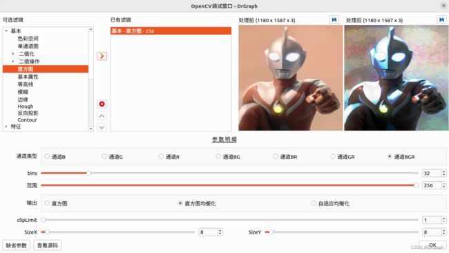
直方图均衡化（Histogram Equalization）是一种图像增强技术，其目的是通过对图像的直方图进行调整，使得图像的灰度分布更加均匀，从而提高图像的对比度和整体质量。
在直方图均衡化过程中，首先计算图像的直方图，即统计图像中每个灰度级出现的次数或频率。然后，根据直方图的分布情况，对灰度级进行重新映射，使得每个灰度级在整个灰度范围内具有相同的出现概率或频率。
具体实现时，可以通过计算累积直方图来确定灰度级的映射关系。累积直方图表示了灰度级小于等于某个值的像素数量占总像素数量的比例。根据累积直方图，可以将原始的灰度级映射到新的灰度级，使得每个灰度级在新的灰度范围内具有相同的出现概率。
直方图均衡化的效果是使图像的灰度分布更加均匀，从而增强图像的对比度和细节。它可以用于改善图像的视觉效果，特别是在低对比度或亮度不均匀的情况下。
需要注意的是，直方图均衡化可能会导致图像的局部信息丢失，因为它是对整个图像进行全局的灰度调整。在实际应用中，需要根据具体情况选择是否使用直方图均衡化以及如何调整参数以获得最佳效果。

自适应直方图均衡化

自适应直方图均衡化（Adaptive Histogram Equalization，AHE）是一种改进的直方图均衡化技术，它在保留图像细节和对比度的同时，对局部区域进行自适应的灰度调整。
传统的直方图均衡化是对整个图像进行全局的灰度变换，可能会导致图像的局部信息丢失。而自适应直方图均衡化则考虑了图像的局部上下文信息，根据每个像素周围的像素分布来调整其灰度级。
自适应直方图均衡化的基本思路如下：
将图像划分为多个子区域（通常是矩形或方形）。
对每个子区域计算其直方图，并进行均衡化操作。
使用均衡化后的子区域直方图对该区域内的像素进行灰度级调整。
通过将图像划分为较小的子区域，可以更好地适应图像中不同区域的灰度分布特征。每个子区域的直方图均衡化操作是独立进行的，从而能够保留图像的局部细节和对比度。
自适应直方图均衡化通常可以提高图像的对比度和细节，尤其在具有亮度不均匀或局部对比度低的情况下效果更为明显。它在图像增强、图像处理和计算机视觉等领域有广泛的应用。
自适应直方图均衡化（Adaptive Histogram Equalization，AHE）和直方图均衡化（Histogram Equalization，HE）都是图像增强技术，用于改善图像的对比度和视觉效果。它们的主要区别在于处理图像的方式。
直方图均衡化是一种全局的方法，它对整幅图像进行均衡化处理。通过计算图像的直方图，然后对灰度级进行重新映射，使得图像的灰度分布更加均匀。这样可以增强图像的对比度，但可能会导致图像的局部细节丢失。
自适应直方图均衡化是对直方图均衡化的改进，它考虑了图像的局部上下文信息。AHE 将图像划分为多个子区域，并对每个子区域进行独立的均衡化处理。这样可以更好地保留图像的局部细节和对比度。
通过将图像划分为较小的子区域，可以更好地适应图像中不同区域的灰度分布特征。每个子区域的直方图均衡化操作是独立进行的，从而能够保留图像的局部细节和对比度。
自适应直方图均衡化在保留图像细节和对比度方面通常比全局的直方图均衡化更有效。它在图像增强、图像处理和计算机视觉等领域有广泛的应用。
其实，说得太多，不知道咋用或用的效果，也是意义不大，至少理解不深，代码倒是很简单

        double clipLimit = GetParamValue_Double(paramIndex++);
        int sizeX = GetParamValue_Int(paramIndex++);
        int sizeY = GetParamValue_Int(paramIndex++);
        auto clahe = createCLAHE(clipLimit, Size(sizeX, sizeY));
        Mat b_hist, g_hist, r_hist;
        if(channelType == 0 || channelType == 3 || channelType == 4 || channelType == 6)    // B
            clahe->apply(mv[0], mv[0]);
        if(channelType == 1 || channelType == 3 || channelType == 5 || channelType == 6)    // G
            clahe->apply(mv[1], mv[1]);
        if(channelType == 2 || channelType == 4 || channelType == 5 || channelType == 6)    // R
            clahe->apply(mv[2], mv[2]);
        merge(mv, dstMat);

反正我是没太理解该咋用，只是用了有图像有变化，这些参数的调整，以后再慢慢理解。