时间序列预测 — BiLSTM-Attention实现单变量负荷预测(Tensorflow)

  专栏链接：https://blog.csdn.net/qq_41921826/category_12495091.html

专栏内容

​ 所有文章提供源代码、数据集、效果可视化

​ 文章多次上领域内容榜、每日必看榜单、全站综合热榜

​

​

​

​

​

​

​

时间序列预测存在的问题

​ 现有的大量方法没有真正的预测未来值，只是用历史数据做验证

​ 利用时间序列分解算法存在信息泄露的问题：有人用emd+lstm对时间序列进行预测，是否存在原理上的问题? - 知乎

---

目录

1 数据处理

1.1 导入库文件

1.2 导入数据集

​1.3 缺失值分析

​2 构造训练数据

3 BiLSTM-Attention模型训练

3.1 搭建Attention模型

3.2 搭建BiLSTM-Attention模型

4 BiLSTM-Attention模型预测

4.1 分量预测

4.2 可视化

---

1 数据处理

1.1 导入库文件

import time
import datetime
import pandas as pd 
import numpy as np 
import matplotlib.pyplot as plt  
from itertools import cycle

import tensorflow as tf 
from sklearn.cluster import KMeans
from sklearn.metrics import r2_score, mean_squared_error, mean_absolute_error, mean_absolute_percentage_error 
from sklearn.preprocessing import MinMaxScaler
from tensorflow.keras.models import Sequential
from tensorflow.keras.layers import Dense, Activation, Dropout, LSTM, GRU, Reshape, BatchNormalization,ConvLSTM2D
from tensorflow.keras.callbacks import ReduceLROnPlateau, EarlyStopping
from keras.optimizers import Adam
from keras.callbacks import EarlyStopping, ModelCheckpoint

# 忽略警告信息
import warnings
warnings.filterwarnings('ignore')  

plt.rcParams['font.sans-serif'] = ['SimHei']     # 显示中文
plt.rcParams['axes.unicode_minus'] = False  # 显示负号
plt.rcParams.update({'font.size':18})  #统一字体字号

1.2 导入数据集

实验数据集采用数据集6：澳大利亚电力负荷与价格预测数据（下载链接），包括数据集包括日期、小时、干球温度、露点温度、湿球温度、湿度、电价、电力负荷特征，时间间隔30min。

# 导入数据
data_raw = pd.read_excel("澳大利亚电力负荷与价格预测数据.xlsx")
data_raw = data_raw[-365*24*6-49:-1].reset_index(drop=True)
data_raw

​对数据进行可视化

from itertools import cycle
# 可视化数据
def visualize_data(data, row, col):
    cycol = cycle('bgrcmk')
    cols = list(data.columns)
    fig, axes = plt.subplots(row, col, figsize=(16, 4))
    fig.tight_layout()
    if row == 1 and col == 1:  # 处理只有1行1列的情况
        axes = [axes]  # 转换为列表，方便统一处理
    for i, ax in enumerate(axes.flat):
        if i < len(cols):
            ax.plot(data.iloc[:,i], c=next(cycol))
            ax.set_title(cols[i])
        else:
            ax.axis('off')  # 如果数据列数小于子图数量，关闭多余的子图
    plt.subplots_adjust(hspace=0.6)
    plt.show()

visualize_data(data_raw.iloc[:,2:], 2, 3)

​因为是单变量负荷预测，只使用电力负荷特征，单独查看部分负荷数据。

data_load = data_raw.iloc[:,-1]
data_load

# 预测结果可视化
plt.figure(dpi=100, figsize=(14, 4))
plt.plot(data_load, markevery=5)
plt.xlabel('时间')
plt.ylabel('负荷')
plt.show()

​​

​1.3 缺失值分析

首先查看数据的信息，发现并没有缺失值

data_raw.info()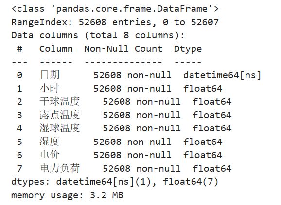

​进一步统计缺失值

data_raw.isnull().sum()

​2 构造训练数据

构造数据前先将数据变为数值类型

data = data_load.values

构造训练数据，也是真正预测未来的关键。首先设置预测的timesteps时间步、predict_steps预测的步长（预测的步长应该比总的预测步长小），length总的预测步长，参数可以根据需要更改。

timesteps = 48*7   #构造x，为48*7个数据,表示每次用前48*7个数据作为一段
predict_steps = 1  #构造y，为1个数据，表示用后1个数据作为一段
length = 48        #预测多步，预测48个数据，每次预测1个
feature_num = 1    #特征个数

通过前timesteps行历史数据预测后面predict_steps个数据，需要对数据集进行滚动划分（也就是前timesteps行的数据和后predict_steps行的数据训练，后面预测时就可通过timesteps行数据预测未来的predict_steps行数据）。这里需要注意的是，因为是单变量预测，特征就是标签，划分数据集时，就用前48*7行当做train_x，第48*7+1行作为train_y，依次滚动划分。

# 构造数据集，用于真正预测未来数据
# 整体的思路也就是，前面通过前timesteps个数据训练后面的predict_steps个未来数据
# 预测时取出前timesteps个数据预测未来的predict_steps个未来数据。
def create_dataset(datasetx, datasety=None, timesteps=96*7, predict_size=12):
    datax = []  # 构造x
    datay = []  # 构造y
    for each in range(len(datasetx) - timesteps - predict_size):
        x = datasetx[each:each + timesteps]
        # 判断是否是单变量分解还是多变量分解
        if datasety is not None:
            y = datasety[each + timesteps:each + timesteps + predict_size]
        else:
            y = datasetx[each + timesteps:each + timesteps + predict_size]
        datax.append(x)
        datay.append(y)
    return datax, datay

​​数据处理前，需要对数据进行归一化，按照上面的方法划分数据，这里返回划分的数据和归一化模型（单变量和多变量的归一化不同，多变量归一化需要将X和Y分开归一化，不然会出现信息泄露的问题），此时的归一化是单变量归一化，函数的定义如下：

# 数据归一化操作
def data_scaler(datax, datay=None, timesteps=36, predict_steps=6):
    # 数据归一化操作
    scaler1 = MinMaxScaler(feature_range=(0, 1))   
    datax = scaler1.fit_transform(datax)
    # 用前面的数据进行训练，留最后的数据进行预测
    # 判断是否是单变量分解还是多变量分解
    if datay is not None:
        scaler2 = MinMaxScaler(feature_range=(0, 1))
        datay = scaler2.fit_transform(datay)
        trainx, trainy = create_dataset(datax, datay, timesteps, predict_steps)
        trainx = np.array(trainx)
        trainy = np.array(trainy)
        return trainx, trainy, scaler1, scaler2
    else:
        trainx, trainy = create_dataset(datax, timesteps=timesteps, predict_size=predict_steps)
        trainx = np.array(trainx)
        trainy = np.array(trainy)
        return trainx, trainy, scaler1, None

然后分解的数据进行划分和归一化。

trainx, trainy, scalerx, scalery = data_scaler(data.reshape(-1, 1), timesteps=timesteps, predict_steps=predict_steps)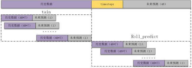

​

3 BiLSTM-Attention模型训练

首先划分训练集、测试集、验证数据：

train_x = trainx[:int(trainx.shape[0] * 0.8)]
train_y = trainy[:int(trainy.shape[0] * 0.8)]
test_x = trainx[int(trainx.shape[0] * 0.8):]
test_y = trainy[int(trainy.shape[0] * 0.8):]
test_x.shape, test_y.shape, train_x.shape, train_y.shape

3.1 搭建Attention模型

参考文章：https://www.cnblogs.com/jiangxinyang/p/9367497.html

(1) Attention思想

深度学习里的Attention model其实模拟的是人脑的注意力模型，举个例子来说，当我们观赏一幅画时，虽然我们可以看到整幅画的全貌，但是在我们深入仔细地观察时，其实眼睛聚焦的就只有很小的一块，这个时候人的大脑主要关注在这一小块图案上，也就是说这个时候人脑对整幅图的关注并不是均衡的，是有一定的权重区分的。这就是深度学习里的Attention Model的核心思想。

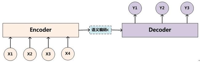
(2) Encoder-Decoder框架

所谓encoder-decoder模型，又叫做编码-解码模型。这是一种应用于seq2seq问题的模型。seq2seq问题简单的说，就是根据一个输入序列x，来生成另一个输出序列y。Encoder-Decoder模型中的编码，就是将输入序列转化成一个固定长度的向量；解码，就是将之前生成的固定向量再转化成输出序列。

Encoder-Decoder（编码-解码）是深度学习中非常常见的一个模型框架，准确的说，Encoder-Decoder并不是一个具体的模型，而是一类框架。Encoder和Decoder部分可以是任意的文字，语音，图像，视频数据，模型可以采用CNN，RNN，BiRNN、LSTM、GRU等等。所以基于Encoder-Decoder，我们可以设计出各种各样的应用算法。

Encoder-Decoder框架可以看作是一种文本处理领域的研究模式，应用场景异常广泛，下图是文本处理领域里常用的Encoder-Decoder框架最抽象的一种表示：

(3) Attention模型 

        在Encoder-Decoder框架中，在预测每一个yi时对应的语义编码c都是一样的，也就意味着序列X中点对输出Y中的每一个点的影响都是相同的。这样就会产生两个弊端：一是语义向量无法完全表示整个序列的信息，再者就是先输入的内容携带的信息会被后输入的信息稀释掉，或者说，被覆盖了。输入序列越长，这个现象就越严重。这就使得在解码的时候一开始就没有获得输入序列足够的信息， 那么解码的准确度自然也就要打个折扣了。

　　为了解决上面的弊端，就需要用到我们的Attention Model（注意力模型）来解决该问题。在机器翻译的时候，让生成词不是只能关注全局的语义编码向量c，而是增加了一个“注意力范围”，表示接下来输出词时候要重点关注输入序列中的哪些部分，然后根据关注的区域来产生下一个输出。模型结构如下：

关于模型的更多介绍可以查阅相关文献，下面给出Attention的代码

# 注意力机制函数
def attention_function(inputs, single_attention_vector=False):    
    # 定义 attention_function 函数，接受输入 inputs 和单一注意力向量标志 single_attention_vector    
    TimeSteps = K.int_shape(inputs)[1]
    # 获取 inputs 的时间步数（序列长度）    
    input_dim = K.int_shape(inputs)[2]
    # 获取 inputs 的特征维度    
    a = Permute((2, 1))(inputs)
    # 将 inputs 的维度进行转置，维度顺序变为 (特征维度, 时间步维度)   
    a = Dense(TimeSteps, activation='softmax')(a)
    # 经过全连接层，输出维度为 (特征维度, 时间步维度)，并使用 softmax 激活函数    
    if single_attention_vector:
        a = Lambda(lambda x: K.mean(x, axis=1))(a)
        # 如果 single_attention_vector 为 True，则对第二个维度进行求平均，得到单一注意力向量
        a = RepeatVector(input_dim)(a)
        # 将单一注意力向量进行复制，使其与 inputs 的维度一致    
    a_probs = Permute((2, 1))(a)
    # 再次将注意力权重进行转置，维度顺序变为 (时间步维度, 特征维度)  
    output_attention_mul = Multiply()([inputs, a_probs])
    # 使用 Multiply 层将 inputs 和注意力权重进行元素级乘法操作    
    return output_attention_mul
    # 返回经过注意力机制处理后的结果 output_attention_mul

3.2 搭建BiLSTM-Attention模型

首先搭建模型的常规操作，然后使用训练数据trainx和trainy进行训练，进行20个epochs的训练，每个batch包含64个样本（建议使用GPU进行训练，增加epochs）。

# 构建LSTM_Attention函数
def LSTM_Attention_train(trainX, trainY, testX, testY, timesteps, predict_steps):
    # 构建BiLSTM模型
    inputs = Input(shape=(timesteps, predict_steps))  # Assuming timesteps=336 and predict_steps=1
​​​​
    BiLSTM_out = Bidirectional(LSTM(128, return_sequences=True, activation="relu"))(inputs)
    Batch_Normalization = BatchNormalization()(BiLSTM_out)
    Drop_out = Dropout(0.1)(Batch_Normalization)
    
    # 构建attention模型
    attention = attention_function(Drop_out)
    Batch_Normalization = BatchNormalization()(attention)
    Drop_out = Dropout(0.1)(Batch_Normalization)
    Flatten_ = Flatten()(Drop_out)
    output = Dropout(0.1)(Flatten_)
    output = Dense(predict_steps, activation='sigmoid')(output)
    model = Model(inputs=[inputs], outputs=output)

    # Compile the model
    model.compile(loss='mean_squared_error', optimizer='adam')

    # Train the model with verbose output
    model.fit(trainX, trainY, epochs=20, batch_size=64, verbose=1, validation_data=(testX, testY))

    return model

然后进行训练，将训练的模型、损失和训练时间保存。

#模型训练
model = BiLSTM_Attention_train(train_x, train_y,test_x, test_y, timesteps, predict_steps)
# 将模型保存为文件
model.save('bilstm_attention.h5')

4 BiLSTM-Attention模型预测

4.1 分量预测

下面介绍文章中最重要，也是真正没有未来特征的情况下预测未来标签的方法。整体的思路也就是取出预测前48*7个数据预测未来的1个数据，然后将1个数据添加进历史数据，再预测1个数据，滚动预测。因为每次只预测1个数据，但是我要预测48个数据，所以采用的就是循环预测48次的思路。

# #滚动predict
# #因为每次只能预测6个数据，但是我要预测6个数据，所以采用的就是循环预测的思路。
# #每次预测的6个数据，添加到数据集中充当预测x，然后在预测新的6个y，再添加到预测x列表中，如此往复,最终预测出48个点。
def predict_BiLSTM_Attention(model, data, timesteps, predict_steps, feature_num, length, scaler):
    predict_xlist = np.array(data).reshape(1, timesteps, feature_num) 
    predict_y = np.array([]).reshape(0, feature_num)  # 初始化为空的二维数组
    print('predict_xlist', predict_xlist.shape)
    
    while len(predict_y) < length:
        # 从最新的predict_xlist取出timesteps个数据，预测新的predict_steps个数据
        predictx = predict_xlist[:,-timesteps:,:]
        # 变换格式，适应模型
        predictx = np.reshape(predictx, (1, timesteps, feature_num)) 
        print('predictx.shape', predictx.shape)
        
        # 预测新值
        lstm_predict = model.predict(predictx)
        print('lstm_predict.shape', lstm_predict.shape)
        
        # 滚动预测
        # 将新预测出来的predict_steps个数据，加入predict_xlist列表，用于下次预测
        print('predict_xlist.shape', predict_xlist.shape)
        predict_xlist = np.concatenate((predict_xlist, lstm_predict), axis=1)
        print('predict_xlist.shape', predict_xlist.shape)
        
        # 预测的结果y，每次预测的6行数据，添加进去，直到预测length个为止
        lstm_predict = scaler.inverse_transform(lstm_predict.reshape(predict_steps, feature_num))
        predict_y = np.concatenate((predict_y, lstm_predict), axis=0)
        print('predict_y', predict_y.shape)
        
    return predict_y

然后对数据进行预测，得到预测结果。

from tensorflow.keras.models import load_model
model = load_model('bilstm_attention.h5')
pre_x = scalerx.fit_transform(data[-48*8:-48].reshape(-1, 1))
y_true = data_load[-48:]
y_predict = predict_BiLSTM_Attention(model, pre_x, timesteps, predict_steps, feature_num, length, scalerx)

4.2 可视化

对预测的结果进行可视化并计算误差。

# 预测并计算误差和可视化
def error_and_plot(y_true,y_predict):
    # 计算误差
    r2 = r2_score(y_true, y_predict)
    rmse = mean_squared_error(y_true, y_predict, squared=False)
    mae = mean_absolute_error(y_true, y_predict)
    mape = mean_absolute_percentage_error(y_true, y_predict)
    print("r2: %.2f\nrmse: %.2f\nmae: %.2f\nmape: %.2f" % (r2, rmse, mae, mape))
    
    # 预测结果可视化
    cycol = cycle('bgrcmk')
    plt.figure(dpi=100, figsize=(14, 5))
    plt.plot(y_true, c=next(cycol), markevery=5)
    plt.plot(y_predict, c=next(cycol), markevery=5)
    plt.legend(['y_true', 'y_predict'])
    plt.xlabel('时间')
    plt.ylabel('功率(kW)')
    plt.show()   
    
    return 0

error_and_plot(y_true.reset_index(drop=True),y_predict)

​