Restricted Boltzmann Machines
Energy-Based Models (EBM)
Energy-based models associate a scalar energy to each configuration of thevariables of interest. Learning corresponds to modifying that energy functionso that its shape has desirable properties. For example, we would likeplausible or desirable configurations to have low energy. Energy-basedprobabilistic models define a probability distribution through an energyfunction, as follows:
(1)![]()
The normalizing factor ![]() is called the partition function by analogywith physical systems.
is called the partition function by analogywith physical systems.
![]()
An energy-based model can be learnt by performing (stochastic) gradientdescent on the empirical negative log-likelihood of the training data. As forthe logistic regression we will first define the log-likelihood and then theloss function as being the negative log-likelihood.

using the stochastic gradient ![]() , where
, where ![]() are the parameters of the model.
are the parameters of the model.
EBMs with Hidden Units
In many cases of interest, we do not observe the example ![]() fully, or wewant to introduce some non-observed variables to increase the expressive powerof the model. So we consider an observed part (still denoted
fully, or wewant to introduce some non-observed variables to increase the expressive powerof the model. So we consider an observed part (still denoted ![]() here) and ahidden part
here) and ahidden part ![]() . We can then write:
. We can then write:
(2)
In such cases, to map this formulation to one similar to Eq. (1), weintroduce the notation (inspired from physics) of free energy, defined asfollows:
(3)![]()
which allows us to write,

The data negative log-likelihood gradient then has a particularly interestingform.
(4)
Notice that the above gradient contains two terms, which are referred to asthe positive and negative phase. The terms positive and negative donot refer to the sign of each term in the equation, but rather reflect theireffect on the probability density defined by the model. The first termincreases the probability of training data (by reducing the corresponding freeenergy), while the second term decreases the probability of samples generatedby the model.
It is usually difficult to determine this gradient analytically, as itinvolves the computation of![]() . This isnothing less than an expectation over all possible configurations of the input
. This isnothing less than an expectation over all possible configurations of the input![]() (under the distribution
(under the distribution ![]() formed by the model) !
formed by the model) !
The first step in making this computation tractable is to estimate theexpectation using a fixed number of model samples. Samples used to estimate thenegative phase gradient are referred to as negative particles, which aredenoted as ![]() . The gradient can then be written as:
. The gradient can then be written as:
(5)![]()
where we would ideally like elements ![]() of
of ![]() to be sampledaccording to
to be sampledaccording to ![]() (i.e. we are doing Monte-Carlo).With the above formula, we almost have a pratical, stochastic algorithm forlearning an EBM. The only missing ingredient is how to extract these negativeparticles
(i.e. we are doing Monte-Carlo).With the above formula, we almost have a pratical, stochastic algorithm forlearning an EBM. The only missing ingredient is how to extract these negativeparticles ![]() . While the statistical literature abounds withsampling methods, Markov Chain Monte Carlo methods are especially well suitedfor models such as the Restricted Boltzmann Machines (RBM), a specific type ofEBM.
. While the statistical literature abounds withsampling methods, Markov Chain Monte Carlo methods are especially well suitedfor models such as the Restricted Boltzmann Machines (RBM), a specific type ofEBM.
Restricted Boltzmann Machines (RBM)
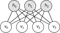
Boltzmann Machines (BMs) are a particular form of log-linear Markov Random Field (MRF),i.e., for which the energy function is linear in its free parameters. To makethem powerful enough to represent complicated distributions (i.e., go from thelimited parametric setting to a non-parametric one), we consider that some ofthe variables are never observed (they are called hidden). By having more hiddenvariables (also called hidden units), we can increase the modeling capacityof the Boltzmann Machine (BM).Restricted Boltzmann Machines further restrict BMs tothose without visible-visible and hidden-hidden connections. A graphicaldepiction of an RBM is shown below.
The energy function ![]() of an RBM is defined as:
of an RBM is defined as:
(6)![]()
where ![]() represents the weights connecting hidden and visible units and
represents the weights connecting hidden and visible units and![]() ,
, ![]() are the offsets of the visible and hidden layersrespectively.
are the offsets of the visible and hidden layersrespectively.
This translates directly to the following free energy formula:
![]()
Because of the specific structure of RBMs, visible and hidden units areconditionally independent given one-another. Using this property, we canwrite:

RBMs with binary units
In the commonly studied case of using binary units (where ![]() and
and ![]() ), we obtain from Eq. (6) and (2), a probabilisticversion of the usual neuron activation function:
), we obtain from Eq. (6) and (2), a probabilisticversion of the usual neuron activation function:
(7)![]()
(8)![]()
The free energy of an RBM with binary units further simplifies to:
(9)
Update Equations with Binary Units
Combining Eqs. (5) with (9), we obtain thefollowing log-likelihood gradients for an RBM with binary units:
(10)
For a more detailed derivation of these equations, we refer the reader to thefollowing page,or to section 5 of Learning Deep Architectures for AI. We will however not use these formulas, but rather get the gradient using Theano T.gradfrom equation (4).
Sampling in an RBM
Samples of ![]() can be obtained by running a Markov chain toconvergence, using Gibbs sampling as the transition operator.
can be obtained by running a Markov chain toconvergence, using Gibbs sampling as the transition operator.
Gibbs sampling of the joint of N random variables ![]() is done through a sequence of N sampling sub-steps of the form
is done through a sequence of N sampling sub-steps of the form![]() where
where ![]() contains the
contains the ![]() other random variables in
other random variables in ![]() excluding
excluding ![]() .
.
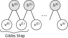
For RBMs, ![]() consists of the set of visible and hidden units. However,since they are conditionally independent, one can perform block Gibbssampling. In this setting, visible units are sampled simultaneously givenfixed values of the hidden units. Similarly, hidden units are sampledsimultaneously given the visibles. A step in the Markov chain is thus taken asfollows:
consists of the set of visible and hidden units. However,since they are conditionally independent, one can perform block Gibbssampling. In this setting, visible units are sampled simultaneously givenfixed values of the hidden units. Similarly, hidden units are sampledsimultaneously given the visibles. A step in the Markov chain is thus taken asfollows:

where ![]() refers to the set of all hidden units at the n-th step ofthe Markov chain. What it means is that, for example,
refers to the set of all hidden units at the n-th step ofthe Markov chain. What it means is that, for example, ![]() israndomly chosen to be 1 (versus 0) with probability
israndomly chosen to be 1 (versus 0) with probability ![]() ,and similarly,
,and similarly,![]() israndomly chosen to be 1 (versus 0) with probability
israndomly chosen to be 1 (versus 0) with probability ![]() .
.
This can be illustrated graphically:
As ![]() , samples
, samples ![]() areguaranteed to be accurate samples of
areguaranteed to be accurate samples of ![]() .
.
In theory, each parameter update in the learning process would require runningone such chain to convergence. It is needless to say that doing so would beprohibitively expensive. As such, several algorithms have been devised forRBMs, in order to efficiently sample from ![]() during the learningprocess.
during the learningprocess.
Contrastive Divergence (CD-k)
Contrastive Divergence uses two tricks to speed up the sampling process:
- since we eventually want
 (the true, underlyingdistribution of the data), we initialize the Markov chain with a trainingexample (i.e., from a distribution that is expected to be close to
  ,so that the chain will be already close to having converged to its final distribution ).
 - CD does not wait for the chain to converge. Samples are obtained after onlyk-steps of Gibbs sampling. In pratice,
 has been shown to worksurprisingly well.
Persistent CD
Persistent CD [Tieleman08] uses another approximation for sampling from![]() . It relies on a single Markov chain, which has a persistentstate (i.e., not restarting a chain for each observed example). For eachparameter update, we extract new samples by simply running the chain fork-steps. The state of the chain is then preserved for subsequent updates.
. It relies on a single Markov chain, which has a persistentstate (i.e., not restarting a chain for each observed example). For eachparameter update, we extract new samples by simply running the chain fork-steps. The state of the chain is then preserved for subsequent updates.
The general intuition is that if parameter updates are small enough comparedto the mixing rate of the chain, the Markov chain should be able to “catch up”to changes in the model.