This series of articles are the study notes of " Machine Learning ", by Prof. Andrew Ng., Stanford University. This article is the notes of week 4, Neural Networks Representation Part II. It contains topics about forward propagation, features of Neural Network and other network architectures.
Neural Networks Representation Part II
1. Model representation II
In the last section, we gave a mathematical definition of how to represent or how to compute the hypotheses used by Neural Network. In this video, I like show you how to actually carry out that computation efficiently, and that is show you a vector rise implementation. And second, and more importantly, I want to start giving you intuition about why these neural network representations might be a good idea and how they can help us to learn complex nonlinear hypotheses.
Forward propagation: Vectorized implementation
Consider this neural network. Previously we said that the sequence of steps that we need in order to compute the output of a hypotheses is these equations given on the left where we compute the activation values of the three hidden uses and then we use those to compute the final output of our hypotheses h of x.
Now, I'm going to define a few extra terms. So, this term that I'm underlining here, I'm going to define that to be z
1
(2).
So that we have that
a
1
(2)=
g(z
1
(2))


Now if you look at this gray block of numbers, you may notice that that block of numbers corresponds suspiciously similar to the matrix vector operation, matrix vector multiplication of θ(1) times the vector x. Using this observation we're going to be able to vectorize this computation of the neural network.
This process of computing hθ(x) is also called forward propagation and is called that because we start of with the activations of the input-units and then we sort of forward-propagate that to the hidden layer and compute the activations of the hidden layer and then we sort of forward propagate that and compute the activations of the output layer, but this process of computing the activations from the input then the hidden then the output layer, and that's also called forward propagation and what we just did is we just worked out a vector wise implementation of this procedure. So, if you implement it using these equations that we have on the right, these would give you an efficient way or both of the efficient way of computing h of x.
Neural Network learning its own features
This forward propagation view also helps us to understand what Neural Networks might be doing and why they might help us to learn interesting nonlinear hypotheses.
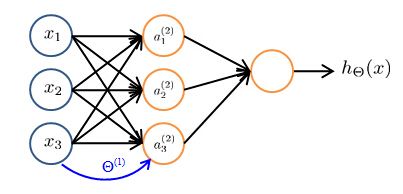
Consider the following neural network and let's say I cover up the left path of this picture for now. If you look at what's left in this picture. This looks a lot like logistic regression where what we're doing is we're using that note, that's just the logistic regression unit and we're using that to make a prediction
hθ
(x). And concretely what the hypotheses is outputting is
hθ
(x) is going to be equal to g which is my sigmoid activation function times theta 0 times
a
0 is equal to 1 plus theta 1 plus theta 2 times
a
2 plus theta 3 times
a
3 whether values
a
1,
a
2,
a
3 are those given by these three given units.

Now, to be actually consistent to my early notation. Actually, we need to, fill in these superscript 2, also have these indices 1 there because I have only one output unit, but if you focus on the blue parts of the notation.

Neural network is just like logistic regression using new features a1, a2, a3
This looks awfully like the standard logistic regression model, except that I now have a capital theta instead of lower case theta. And what this is doing is just logistic regression. But where the features fed into logistic regression are these values computed by the hidden layer. Just to say that again,
what this neural network is doing is just like logistic regression, except that rather than using the original features
x1, x2, x3 ,is using these new features a1, a2, a3.
Neural network is going to learn its own features, a1, a2, a3

And the cool thing about this, is that the features a1, a2, a3, they themselves are learned as functions of the input. Concretely, the function mapping from layer 1 to layer 2, that is determined by some other set of parameters, theta 1. So it's as if the neural network, instead of being constrained to feed the features x1, x2, x3 to logistic regression. It gets to learn its own features,a1, a2, a3, to feed into the logistic regression and as you can imagine depending onwhat parameters it chooses forθ(1) . You can learn some pretty interesting and complex features and therefore you can end up with a better hypotheses than if you were constrained to use the raw features x1, x2, x3 or if you will constrain to say choose the polynomial terms, you know, x1, x2, x3, and so on. But instead, this algorithm has the flexibility to try to learn whatever features at once, using these a1, a2, a3 in order to feed into this last unit that's essentially a logistic regression here.
Other network architectures
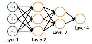
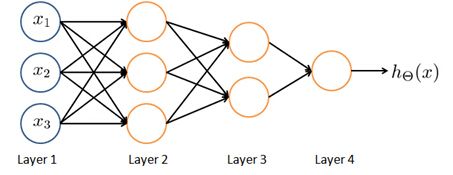
You can have neural networks with other types of diagrams as well, and the way that neural networks are connected, that's called the architecture. So the term architecture refers to how the different neurons are connected to each other. This is an example of a different neural network architecture and once again you may be able to get this intuition of how the second layer, here we have three heading units that are computing some complex function maybe of the input layer, and then the third layer can take the second layer's features and compute even more complex features in layer three so that by the time you get to the output layer, layer four, you can have even more complex features of what you are able to compute in layer three and so get very interesting nonlinear hypotheses. By the way, in a network like this, layer one, this is called an input layer. Layer four is still our output layer, and this network has two hidden layers. So anything that's not an input layer or an output layer is called a hidden layer.

Quiz:
