
This project was carried out by Garance Bruneau, Sorya Dubray and Axel Murguet as part of Professor Filliat's course on Mobile Robotics at ENSTA ParisTech. This course is a significant part of our last year of graduate engineering studies for our specialism: "Robotics and Embedded Systems".
As we are highly interested in SLAM-related issues, which are at the core of Professor Filliat's course, we came out with the choice of implementing aMonoSLAM for the project part of the course. Moreover, this subject make use of other courses we attended this year at ENSTA ParisTech, such asProfessor Manzanera's course on Computer Vision. Last but not least, we wanted to:
- Have fun with a somewhat challenging project... and doing it from scratch;
- Be able to work on real life signals rather than on a simulation project, with unnatural noises;
- To get a hands-on experience, in particular about calibration-related issues.
Therefore, we chose to coarsely reproduce Professor Davison's 2003 paper "Real-Time Simultaneous Localisation and Mapping with a Single Camera", without the real-time aspect.
Feel free to contact us at:
- murguet at free dot fr
- garance dot bruneau at gmail dot com
- dubray dot sory at gmail dot com
Basics - Structure from motion [top]
What is MonoSLAM? [top]
SLAM is a generic acronym in robotics standing for Simultaneous Localization and Mapping. There are several ways of solving this class of problems.
One of these methods is MonoSLAM, with a camera as sole and unique sensor. This belongs to the more general set of visual SLAM algorithms. Compared to more usual techniques, there is no odomotry nor IMU information available here, but only 2D data. Still, from that, we need to recover full 3D information such as the camera position and orientation, and the position of the landmarks (the map is made of the set of landmarks).
Depth has so to be estimated through the camera motion. However, the use of ego motion in order to fully qualify the landmarks makes MonoSLAM more difficult than traditional SLAM methods. Indeed, estimating a new landmark position is tightly linked to the camera motion estimation. This is an occurence of the class of problems referred to as "structure from motion".
Overview [top]
To get an idea on how MonoSLAM is working, we can roughly introduce it through a few remarks.
- SLAM in a 3D environment → Need of 3D landmarks;
- Camera-based method → Use of visual 2D interest points;
- Camera gives 2D interest points → No depth information;
- How to get depth? → By using camera motion;
- How to estimate camera motion? → By using 3D landmarks!
So it leads to the following conclusions:
- 3D landmark = 2D interest point + depth;
- A few initial landmarks must be given to the algorithm (otherwise camera motion cannot be estimated at the beginning, and no landmark can be placed)
- After an initialization phase, the MonoSLAM algorithm is an iterative process in which:
- 2D interest points must evolve into 3D landmarks when the estimate of their depth is good enough;
- 3D landmarks contibute to estimation of the state (camera and map).
The following picture sums up the global architecture of the algorithm, introducing the basic blocks we are going to explain in further details.
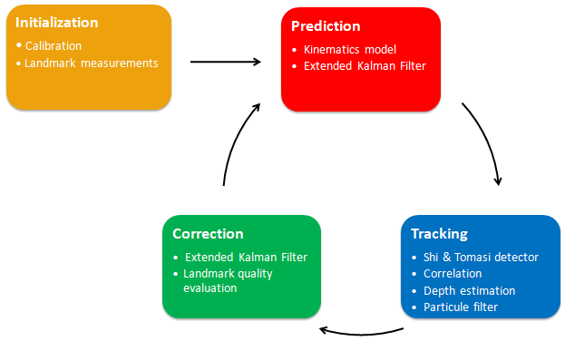
Details of the implementation [top]
The notations and equations are those of Davison's 2003 paper.
The camera and map state is estimated through an Extented Kalman Filter (EKF). After an initialization step, this filter performs a model-based prediction, compares it to the measurements (camera data), and thus applies a correction on the global state according to the innovation.
Initialization [top]
To use the camera data, it is necessary to know its parameters such as resolution, focal length, CMOS sensor dimension... To get a fine estimation of them, one is supposed to perform a calibration step. Automatic tools such as the "Camera Calibration Toolbox for Matlab" freely available here can be used.
As mentionned before, a few initial landmarks have to be given. Currently, this step is done manually. But it could be done in an automated manner, by using an object of known size (as a A4 sheet of paper) at the beginning for instance.
Prediction [top]
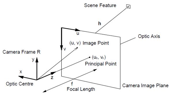
The world frame and the camera frame are described in the following picture (from Davison's "Real-Time Simultaneous Localisation and Mapping with a Single Camera"):

The camera state is described by its:
- Position (r)
- Orientation (using a quaternion, q)
- Linear speeds (v)
- Angular speeds (ω)
Leading thus to a 13-dimension camera state vector Xv.
As we use an EKF, it means that we must have a model. As the camera could be embedded on any type of robot, or even a human being, the only model we can have is a kinematic one (and not a dynamic one). So, using a constant velocity model, the evolution of the camera would be given by the following set of equations:
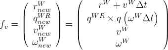
This model allows only constant velocity movement. However, this is not very realistic: indeed, there is no reason for the camera to move this way. That is why we must add a noise as a way to allow for "errors" to be accepted (i.e., changes in the direction, speed, etc). This is necessary for the EKF to assess the confidence into its estimates.
An additive noise model (with random gaussian noise added on each state component) is very common, but we used a non-linear, acceleration-based noise model. In order to enable several trajectories around the previous one, we consider the linear and angular accelerations to be given by random zero-mean gaussian variables. The standard deviation of these variables allows to tune how uneven the motion can be.
Linear acceleration is represented by the stochastic variable "a":
![]()
Angular acceleration is represented by the stochastic variable "α":
![]()
Leading to the noise vector "n" (with covariance matrix "Pn"):
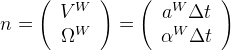
Introducing this noise, the kinematic model becomes:
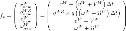
This allows the predition to gives results such that (from "Real-Time 3D SLAM with Wide-Angle Vision"):
The prediction step randomly chooses one trajectory among these possibilities, and then, if necessary, the correction step will bring the system back in tracks.
The complete state (X) of the EKF is formed by the camera state (Xv) and the landmark 3D positions (Yi).

Given the previous model, the computation of the prediction is easy to obtain. Nonetheless, the computation of the uncertainty (represented by the covariance matrix) is more difficult. Symbolic computation has to be used to compute the jacobians, especially for the quaternion part of the function. These jacobians are used for the filter covariance "P" update:
![]()
In addition to the computation of derivatives, the quaternion has to be kept unitary. Therefore, an additionnal normalization step has to be performed at each iteration, and this has to be taken into account in the jacobians.
Tracking [top]
Interest points management
Landmarks are identified from interest points detection. The Shi and Thomasi detector is used to define salient points. The detection is based on local extrema of the gradient analysis of 15x15 pixels patches. The eigenvalues of the following matrix are used to assess the quality of a potential interest point,through a threshold (note that this is a symetric, definite positive matrix):

When a new interest point is identified, it is attached its neighboorhood, namely its 15x15 pixels patch, to describe this point. To increase the robustness of the detection (regarding the illumination), the patch is normalized.
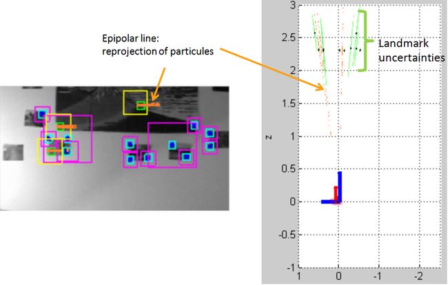
There is no depth information from a single image. We need motion to recover this last piece of information. This is done thanks to a particule filter. When an interest point is selected, we only know that this point belongs to a certain line, called the epipolar line. To estimate where the point lies on this epipolar line, the line is uniformly sampled by a given number of particules, where each particule represents a depth hypothesis. Of course, it is not possible with such a technique to sample the complete epipolar line, as it is semi-infinite. A maximal depth hypothesis, related to the size of the environnement, limits the search zone.
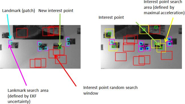
When an interest point has been registered, meaning that its patch and epipolar line are known, the algorithm tries to match it in the subsequent pictures. For an interest point (without any depth information), the tracking simply relies on correlation over a window. The size of this windows is constant, defined by a maximal acceleration (in terms of pixels).
Interest points moving out of the image or weakly matched are discarded.
During the tracking, after the correlation has matched an interest point, all the particules associated to this point are reprojected in the picture. Resampling is performed to promote hypothesis best-linked to the correlation result, but 25% of the particules are resampled uniformly to avoid early convergence. When the variance of the depth hypotheses shrinks below a threshold, the estimation is considered reliable. The interest point is then attached a depth and becames a landmark, with a large uncertainty along the epipolar line (to allow the EKF to modify its position easily if necessary).
Landmarks tracking
Compared to the interest point management (initialization, tracking, depth estimation and upgrade as landmark), which was previously explained, landmarks tracking is much easier.
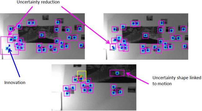
The EKF prediction gives an estimate of the camera position and orientation, as well as uncertainties on these quantities and on the landmarks position. The position and orientation of the camera, relative to the landmarks postion, allow to predict how the landmarks will be projected onto the image plane, along with an uncertainty area. It is worth noticing that both the uncertainty of the camera (position and orientation) and the one of the landmark position are taken into account to compute this uncertainty area. The larger the uncertainty is, the wider the search area is in the new picture. Then, the search is simply performed by correlation within this area. The difference between the EKF prediction and the camera observation gives the innovation signal of the filter.
At least one landmark must always be visible while the algorithm is running. Thus, as soon as the number of visible landmarks falls below a chosen number, a search procedure is launched, in order to identify new interest points (landmarks to be). This is simply achieved by searching interest points in randomly drawn windows. The only constraint on these windows is they have to be far away from the currently tracked landmarks and interest points. Otherwise, no effort is spent in trying to pick up interest points in the most useful place for the algorithm (i.e., related to the motion of the camera for instance).
Correction [top]
The innovation signal is at the core of the EKF correction step, which affects the whole state vector. We previously explained how the innovation signal is obtained, without any details concerning the projection. This aspect and the observation model will be discussed here.
The simple pinhole camera model is used to perform reprojection. No distorsion correction is applied here.
For a landmark Yi (described by its coordinates in the world frame), we have to express its position relatively to the camera. We can find the camera position "r" in the state vector, and the rotation matrix from the world frame to the camera frame "RRW" has to be built from the quaternion "q" of the state vector. The landmark expressed in the camera frame is thus given by:
![]()
And the pinhole camera model leads to ("f" being the focal length, "ku" and "kv" factors to be taken into account CMOS captor dimensions, from Davison's "SLAM with a Single Camera"):
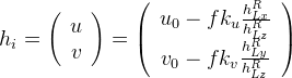
As previously, symbolic computation should be used to compute the jacobians:
![]()
Correction is based on the innovation. A simple additive noise is finally added to the observation model. This enable to tune the confidence of the EKF towards the observations.
To increase the robustness of the correction algorithm, landmarks weakly matched (bad correlation results) or unmatched (not seen when they are predicted to be seen) along several frames are removed from the map. This way, occulted landmarks or parasitic reflections do not disturb the altorithm. Indeed, the EKF is very likely to be lost if the landmark assotiation is bad. Therefore, unrealiable matching must not be used.
Results [top]
Raw data [top]
Our implementation was tested by trying to map the following piece of room. As one can see on the following picture, there is a corner we expect the algorithm to reproduce.

The MonoSLAM raw test video can be downloaded here (MPEG4-Xvid format).
Video anotation explanation [top]
Here are some explanations about video annotation:
On the right side of the video frames, one can see the 3D view of the map (top view). The world frame axes are represented in blue, the camera frame axes in red.
Video results [top]
The videos below show two runs of the algorithm, the first one is succesfull, the second is not. As the implementation is not real-time, both were processed back to the frame rate of the original video.
In this run, there always is at least one visible landmark, which prevent the filter from being lost. This is due to the fast convergence of the particule filters in this case. One can see that the camera movements are well retrieved, for instance when going closer to the wall and back. The changes in the camera uncertainty ellipsoid are strongly linked to the number of visible landmarks and to how discriminating the motion is (translation is good, rotation is more difficult to manage).
The MonoSLAM result video can be downloaded here (MPEG4-Xvid format).
In this run, the particule filters did not converge quickly enough, and therefore the system ends in a state where there is no visible landmark. That is why there is no innovation, and no way to correct the predicted motion. The filter has no information telling that the camera stops going up and starts going down. Therefore, it "thinks" that the camera keeps its upward movement, and does not try to retrieve the knwon landmarks (as it does not expect them to be seen). This is how it creates new interest points instead of recognizing landmarks, and is lost without any hope of recovering (growing red uncertainty ellipsoid at the end of the video).
The MonoSLAM divergence video can be downloaded here (MPEG4-Xvid format).
Limitations [top]
From a theoritical point of view, there are several limits to this approach:
- It is based on a EKF, which is a rough linearization (first order only). Is it thus prone to divergence. Moreover, one needs to tune the noise parameters, which can only be done by trials. Finally, it is very difficult for the filter to recover from a false landmark association. To help with this issue, we use many landmarks and we remove the "bad" landmarks.
- The particule filter can be very slow to converge without good discriminant movements (such as translations), which can lead towards divergence.
- This approch is based on visual interest points, and therefore is not possible in uniform environments.
On top of these issues, we faced some more practical problems, mainly linked to the video recorder:
- The video recorder we had (only a camera, not a real video recorder) was not suited for this use:
- The auto-focus changes the focal length automatically. Calibration was consequently not meaningful. That is why we used the camera in a restraint range of distance, to remain close to the valid region of the observation model (which uses a constant focal length).
The camera parameters in the observation model were tuned manually to get an acceptable reprojection in the first pictures (based on the manually measured landmarks). - To reduce the distorsion, we decided to zoom in. The drawback of this method is a limited viewing-angle, making mapping more difficult (only a very limited area of the room is visible at a time).
- The interlaced capture mode leads to blur in case of fast motion. By chance, the robusteness of the tracking overcame this limitation easily.
- The automatic exposure capture could lead to significant change in the illumination of the landmarks. The normalization step of the patches-based description is a efficient way to make the traking robust regarding this issue.
- The auto-focus changes the focal length automatically. Calibration was consequently not meaningful. That is why we used the camera in a restraint range of distance, to remain close to the valid region of the observation model (which uses a constant focal length).
- Initial landmarks position: without a bench test, we could only have very rough measurements, which limits the precision of the whole system. Practically, this problem was not as bad as one could think it would be.
Conclusion [top]
Thanks to this project, we got a chance to learn a lot about SLAM, about the issues you have to face when implementing a real demonstrator, in particular with a standard camera, and about all these details no one ever talks about but which can ask for quite some time to work on...
To sum up, we were very happy of this project which was a lot of fun, and we are glad that we got a working result under these realistic conditions, and that with little time and no specific tools.
A few ideas to go further...
- Using "inverse depth" parametrization
- Using an UKF (Unscented Kalman Filter) instead of the EKF
- Rao-Blackwellizing the filter (see FastSLAM)
- Using the optical flow
Bibliography [top]
- "Real-Time Simultaneous Localisation and Mapping with a Single Camera", Andrew J. Davison, 2003
- "Good Features to Track", J. Shi and C. Tomasi, 1994
- "SLAM with a Single Camera", Andrew J. Davison, 2002
- "Real-Time 3D SLAM with Wide-Angle Vision", Andrew J. Davison, Yolanda González Cid, Nobuyuki Kita, 2004