吴恩达深度学习总结

Deep learning

Use open source code

1. Use architectures of networks published in the literature
2. Use open source implementation if possible
3. Use pretrained models and fine-tune on your dataset

神经网络和深度学习

1. LSF

   J=0; dw1=0; dw2=0; db=0;
   for i = 1 to m
   z(i) = wx(i)+b;
   a(i) = sigmoid(z(i));
   J += -[y(i)log(a(i))+(1-y(i)）log(1-a(i));
   dz(i) = a(i)-y(i);
   dw1 += x1(i)dz(i);
   dw2 += x2(i)dz(i);
   db += dz(i);
   J /= m;
   dw1 /= m;
   dw2 /= m;
   db /= m;
   w=w-alpha*dw
   b=b-alpha*db
   
   
   Vectorize implementation
    Z = np.dot(w.T,x)
    A = sigmoid(Z)
    dZ = A-Y
    dw = 1/m*X*(dz.T)
    db = 1/m*np.sum(dz)
    w = w - alpha*dw
    b = b - alpha*db                   

   funtion_normalizeRow
   
       x_ = np.linalg.norm(x, axis=1, keepdims = True)
   
       x = x / x_
   
       return x
   
   

   A trick when you want to flatten a matrix X of shape (a,b,c,d) to a matrix X_flatten of shape (b∗∗c∗∗d, a) is to use:

   X_flatten = X.reshape(X.shape[0], -1).T      # X.T is the transpose of X
   

   What you need to remember:

   Common steps for pre-processing a new dataset are:

   • Figure out the dimensions and shapes of the problem (m_train, m_test, num_px, ...)
   • Reshape the datasets such that each example is now a vector of size (num_px * num_px * 3, 1)
   • "Standardize" the data

2. NN

    dZ2 = A2 - Y
       dW2 = 1/m*dZ2.dot(A1.T)
       db2 = 1/m*np.sum(dZ2,axis = 1, keepdims = True)
       dZ1 = W2.T.dot(dZ2) * (1 - np.power(A1, 2))
       dW1 = dZ1.dot(X.T)
       db1 = 1/m*np.sum(dZ1, axis = 1, keepdims = True)

3. 多层NN

   ​ Note that for every forward function, there is a corresponding backward function. That is why at every step of your forward module you will be storing some values in a cache.

   Several layers have several activation functions, In deep learning, the "[LINEAR->ACTIVATION]" computation is counted as a single layer in the neural network, not two layers.

rule: Idea to Code to Experiment (circle)

改善深层神经网络

正则化：旨在消除方差以及偏差的一系列方法， 包括

1. 数据扩增（用于修正方差）
2. L2正则化
3. dropout正则化（用于修正方差）

一些需要考虑的问题

1. 小数据时代七三分或者六二二分是个不错的选择，在大数据时代各个数据集的比例可能需要变成98%：1%：1%，甚至训练集的比例更大。

2. 确保验证集和测试集来自于同一分布

3. 测试集的目的是对最终所选定的神经网络系统做出无偏估计，如果不需要无偏估计也可以不设置测试集。

4. 机器学习比较在意bias-variance trade-off,但深度学习的误差很少权衡两者，我们总是分别讨论偏差或者方差，却很少谈及偏差和方差的权衡问题

5. 采用双边误差更逼近导数：使用泰勒定理推导

1. 详细介绍

   1. 执行方面的小建议：使用新的cost函数，包含第二个正则化项。
   2. dropout本质：每次都训练不同的子集，均摊各个权重，且只使用在训练期，前向和后向都使用
   3. L2正则化，缺点是必须尝试很多正则化参数λ，early stopping 的优点是只运行一次梯度下降，你可以找出W 的较小值，中间值和较大值，（实际中用的不多）

2. 使用权重初始化解决爆炸或者坍塌

   原因：L>I，产生exploding，L<1, 产生vanish
   \[ cost = W^{L-1}X \]
   因此初始权重尽可能逼近1，以下为普遍法则

   1. 如果是常用relu激活函数，W = np.random.randn(shape)*np.sqrt(2/n^(L-1))
   2. 如果是tanh， np.sqrt(1/n^(L-1)) or np.sqrt(2/(n^(L-1) + n^L)

3. 梯度检验注意事项

   1. 只用在debug
   2. 带上正则化
   3. 不能与dropout同时使用
   4. 在这样一种情况：只有W和b接近0的时候BP才是正确的。在随机初始化过程中，运行梯度检验，然后再训练网络

dropout 和L2正则化使用代码

# Forward propagation: LINEAR -> RELU -> LINEAR -> RELU -> LINEAR -> SIGMOID.
        if keep_prob == 1:
            a3, cache = forward_propagation(X, parameters)
        elif keep_prob < 1:
            a3, cache = forward_propagation_with_dropout(X, parameters, keep_prob)
        
        # Cost function
        if lambd == 0:
            cost = compute_cost(a3, Y)
        else:
            cost = compute_cost_with_regularization(a3, Y, parameters, lambd)
            
        # Backward propagation.
        assert(lambd==0 or keep_prob==1)    # it is possible to use both L2 regularization and dropout, 
                                            # but this assignment will only explore one at a time
        if lambd == 0 and keep_prob == 1:
            grads = backward_propagation(X, Y, cache)
        elif lambd != 0:
            grads = backward_propagation_with_regularization(X, Y, cache, lambd)
        elif keep_prob < 1:
            grads = backward_propagation_with_dropout(X, Y, cache, keep_prob)
            
            
               
            
            FORWARD_PROPAGATION
    ### START CODE HERE ### (approx. 4 lines)         # Steps 1-4 below correspond to the Steps 1-4 described above. 
    D1 = np.random.rand(A1.shape[0], A1.shape[1])                                         # Step 1: initialize matrix D1 = np.random.rand(..., ...)
    D1 = D1 < keep_prob                                         # Step 2: convert entries of D1 to 0 or 1 (using keep_prob as the threshold)
    A1 = D1 * A1                                         # Step 3: shut down some neurons of A1
    A1 = A1 / keep_prob                                         # Step 4: scale the value of neurons
    
    
    
            BACKWARD_PROPAGATION
     ### START CODE HERE ### (≈ 2 lines of code)
    dA2 = D2 * dA2              # Step 1: Apply mask D2 to shut down the same neurons as during the forward propagation
    dA2 = dA2 / keep_prob              # Step 2: Scale the value of neurons that haven't been shut dow

梯度检验代码

To compute J_plus[i]:
    Set θ+ to np.copy(parameters_values)
    Set θ+i to θ+i+ε
    Calculate J+i using to forward_propagation_n(x, y, vector_to_dictionary(θ+ )).
To compute J_minus[i]: do the same thing with θ−
Compute gradapprox[i]=J+i−J−i2ε

    for i in range(num_parameters): 
        
        # Compute J_plus[i]. Inputs: "parameters_values, epsilon". Output = "J_plus[i]".
        # "_" is used because the function you have to outputs two parameters but we only care about the first one
        ### START CODE HERE ### (approx. 3 lines)
        theta_plus = np.copy(parameters_values)
        theta_plus[i][0] += epsilon
        J_plus[i], _ = forward_propagation_n(X, Y ,vector_to_dictionary(theta_plus))
        ### END CODE HERE ###
        
        # Compute J_minus[i]. Inputs: "parameters_values, epsilon". Output = "J_minus[i]".
        ### START CODE HERE ### (approx. 3 lines)
        theta_minus = np.copy(parameters_values)
        theta_minus[i][0] -= epsilon
        J_minus[i], _ = forward_propagation_n(X, Y ,vector_to_dictionary(theta_minus))
        ### END CODE HERE ###
        
        # Compute gradapprox[i]
        ### START CODE HERE ### (approx. 1 line)
        gradapprox[i] = (J_plus[i] - J_minus[i]) / (2 * epsilon)
        ### END CODE HERE ###
    
    # Compare gradapprox to backward propagation gradients by computing difference.
    ### START CODE HERE ### (approx. 1 line)
    numerator = np.linalg.norm(grad - gradapprox) 
    denominator = np.linalg.norm(gradapprox) + np.linalg.norm(grad)
    difference = numerator / denominator
    ### END CODE HERE ###

优化算法

1. mini-batch

   1. 样本集(m<=2000)，使用batch梯度下降
   2. mini-batch尝试几个不同的2次方，一般为64到512，这是考虑到CPU/GPU内存相符

   经测试，批次选择16或者8最好

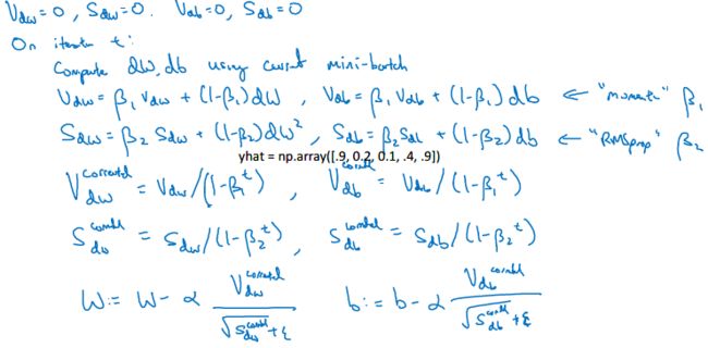
2. Gradient descent with momentum

   动量算法为解决如下情况而出现的，通过平均过去的多少天（由β设定）抵消竖直方向的摆动，而水平方向持续增长。

   动量算法需要尽可能大一点的学习率和复杂一点的数据
   

   \[ \begin{align} v_{dw} = {\beta}v_{dw} \ +\ (1 - \beta)dW\\ v_{db} = \beta v_{db} \ + \ (1-\beta)db\\ W = W\ -\ \alpha v_{dv}, \ \ b = b\ - \ \alpha v_{db} \end{align} \]

3. RMSprop------root mean square prop

   原理与动量算法一致，计算有所区别

4. Adam-----Adaptive Moment Estimation

   结合了以上两种算法

   

   通常， β1取0.9， β2取0.999， ε取10e-8

learning rate decay（衰减率）

局部最优问题

1. 实际上高维空间基本上不存在局部最优（所有都是同一个方向）
2. 真正的问题是缓慢走过平稳段，这也是RMSprop、Momentum 和Adam 能够加速学习算法的地方。

实现代码

1. 梯度

   (Batch) Gradient Descent:
   X = data_input
   Y = labels
   parameters = initialize_parameters(layers_dims)
   for i in range(0, num_iterations):
       # Forward propagation
       a, caches = forward_propagation(X, parameters)
       # Compute cost.
       cost = compute_cost(a, Y)
       # Backward propagation.
       grads = backward_propagation(a, caches, parameters)
       # Update parameters.
       parameters = update_parameters(parameters, grads)
   Stochastic Gradient Descent:
   X = data_input
   Y = labels
   parameters = initialize_parameters(layers_dims)
   for i in range(0, num_iterations):
       for j in range(0, m):
           # Forward propagation
           a, caches = forward_propagation(X[:,j], parameters)
           # Compute cost
           cost = compute_cost(a, Y[:,j])
           # Backward propagation
           grads = backward_propagation(a, caches, parameters)
           # Update parameters.
           parameters = update_parameters(parameters, grads)

2. 批量

   # GRADED FUNCTION: random_mini_batches
   
   def random_mini_batches(X, Y, mini_batch_size = 64, seed = 0):
       """
       Creates a list of random minibatches from (X, Y)
   
       Arguments:
       X -- input data, of shape (input size, number of examples)
       Y -- true "label" vector (1 for blue dot / 0 for red dot), of shape (1, number of examples)
       mini_batch_size -- size of the mini-batches, integer
   
       Returns:
       mini_batches -- list of synchronous (mini_batch_X, mini_batch_Y)
       """
   
       np.random.seed(seed)            # To make your "random" minibatches the same as ours
       m = X.shape[1]                  # number of training examples
       mini_batches = []
   
       # Step 1: Shuffle (X, Y)
       permutation = list(np.random.permutation(m))
       shuffled_X = X[:, permutation]
   
       shuffled_Y = Y[:, permutation].reshape((1,m))
   
       # Step 2: Partition (shuffled_X, shuffled_Y). Minus the end case.
       num_complete_minibatches = math.floor(m/mini_batch_size) # number of mini batches of size mini_batch_size in your partitionning
       for k in range(0, num_complete_minibatches):
           ### START CODE HERE ### (approx. 2 lines)
           mini_batch_X = shuffled_X[:, k*mini_batch_size:(k+1)*mini_batch_size]
           mini_batch_Y = shuffled_Y[:, k*mini_batch_size:(k+1)*mini_batch_size]
           ### END CODE HERE ###
           mini_batch = (mini_batch_X, mini_batch_Y)
           mini_batches.append(mini_batch)
   
       # Handling the end case (last mini-batch < mini_batch_size)
       if m % mini_batch_size != 0:
           ### START CODE HERE ### (approx. 2 lines)
           mini_batch_X = shuffled_X[:, num_compl ete_minibatches * mini_batch_size:]
           mini_batch_Y = shuffled_Y[:, num_complete_minibatches * mini_batch_size:]
           ### END CODE HERE ###
           mini_batch = (mini_batch_X, mini_batch_Y)
           mini_batches.append(mini_batch)
   
       return mini_batches

   至于动量和Adam算法只需修改计算梯度的公式即可。

调试超参数

1. 由粗到细，调参优先级顺序：第一：α， 第二：layer， learning rate decay 第三：β， hidden_units, mini-batch size
2. 坐标选取范围先是用对数。然后在精细
3. 超参数训练的方式：1、熊猫方式 2、鱼子酱方式（优先,如果数据量足够大）
4. batch归一化（应用于Z和a之间），由于需要减去均值，所以b没有意义

Tessorflow 基础

1. create placeholders

   X = tf.placeholder(tf.float32, (n_x, None))
   Y = tf.placeholder(tf.float32, (n_y, None))

2. Initializing the parameters

       tf.set_random_seed(1)                   # so that your "random" numbers match ours
   
       ### START CODE HERE ### (approx. 6 lines of code)
       W1 = tf.get_variable("W1", [25,12288], initializer = tf.contrib.layers.xavier_initializer(seed = 1))
       b1 = tf.get_variable("b1", [25,1], initializer = tf.zeros_initializer())

3. Forward propagation in tensorflow

       Z1 = tf.matmul(W1,X) + b1                                              # Z1 = np.dot(W1, X) + b1
       A1 = tf.nn.relu(Z1)                                              # A1 = relu(Z1)
       Z2 = tf.matmul(W2,A1) + b2                                              # Z2 = np.dot(W2, a1) + b2
       A2 = tf.nn.relu(Z2)                                          # A2 = relu(Z2)
       Z3 = tf.matmul(W3,A2) + b3   
    you don't need a3

4. Compute cost

   It is important to know that the "logits" and "labels" inputs of tf.nn.softmax_cross_entropy_with_logits are expected to be of shape (number of examples, num_classes). We have thus transposed Z3 and Y for you.
   Besides, tf.reduce_mean basically does the summation over the examples.   
   
   
      # to fit the tensorflow requirement for tf.nn.softmax_cross_entropy_with_logits(...,...)
           logits = tf.transpose(Z3)
       labels = tf.transpose(Y)
   
       ### START CODE HERE ### (1 line of code)
       cost = tf.reduce_mean(tf.nn.softmax_cross_entropy_with_logits(logits = logits, labels = labels))
   

5. Backward propagation & parameter updates

   For instance, for gradient descent the optimizer would be:
   
   optimizer = tf.train.GradientDescentOptimizer(learning_rate = learning_rate).minimize(cost)
   To make the optimization you would do:
   
   _ , c = sess.run([optimizer, cost], feed_dict={X: minibatch_X, Y: minibatch_Y})

6. Building the model

   def model(X_train, Y_train, X_test, Y_test, learning_rate = 0.0001,
             num_epochs = 1500, minibatch_size = 32, print_cost = True):

7. Test with your own image

8. ,optimizer = tf.train.GradientDescentOptimizer(learning_rate = learning_rate).minimize(cost),To make the optimization you would do:,,_ , c = sess.run([optimizer, cost], feed_dict={X: minibatch_X, Y: minibatch_Y}),,,

结构化机器学习项目

正交化用于调参

查全率与查准率

我们希望通过在同一分布中设立开发集和测试集，你就可以瞄准你所希望的机器学习团队瞄准的目标。

误差分析

系统性的错误需要纠正

训练数据和开发数据来自不同的分布：

我们来看一个不同的样本，假设训练误差为1%，训练-开发误差为1.5%，但当你开始处理开发集时，错误率上升到10%。这就是数据不匹配（有前提）

处理数据不匹配问题

迁移学习（Transfer learning）

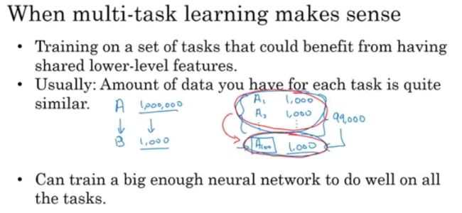
多任务学习（multi-task）

端到端的深度学习（end-to-end learning)

卷积神经网络

why:

1. Parameter compression
2. Sparsity(稀疏)of connections

paper:AlexNet, VGG, LeNet

padding公式：
\[ \frac{n-2*pad-f}s + 1 = n^{'} \\ n^{'}是填充与否后的维度 \]

残差网络（ResNets)（Residual Networks)

解决梯度消失和梯度爆炸问题。

跳跃连接（Skip connection）：它可以从某一层网络层获取激活，然后迅速反馈给另外一层，甚至是神经网络的更深层。我们可以利用跳跃连接构建能够训练深度网络的ResNets，有时深度能够超过100 层，

1x1卷积

最开始用卷积计算的目的就是较少计算量，而卷积核是越小越好，比如一张1000x1000的图片，如果卷积核为1000，采用1个核就能描述图片，那么计算量为1000x1000x1， 如果卷积核为10，那么采用几十个就足以复现图片，计算量不过1000以下，且卷积核的个数越多，所能描述的细节越多，从而遵循小而深。

通过1×1 卷积的简单操作来压缩或保持输入层中的通道数量，甚至是增加通道数量。

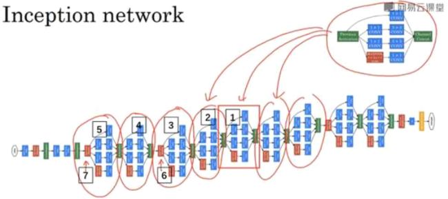
Inception

Inception 网络或Inception 层的作用就是代替人工来确定卷积层中的过滤器类型，或者确定是否需要创建卷积层或池化层（原理是通过计算量的多少判断）.

Common Data augmentation method

1. Mirroring
2. Random Cropping
3. Rotation shearing Local warping(use very little)

Color shifting

​ 对照片的颜色更改更具鲁棒性

​ paper：method:PCA:AlexNet "PCA color augumentation"

Target Detection

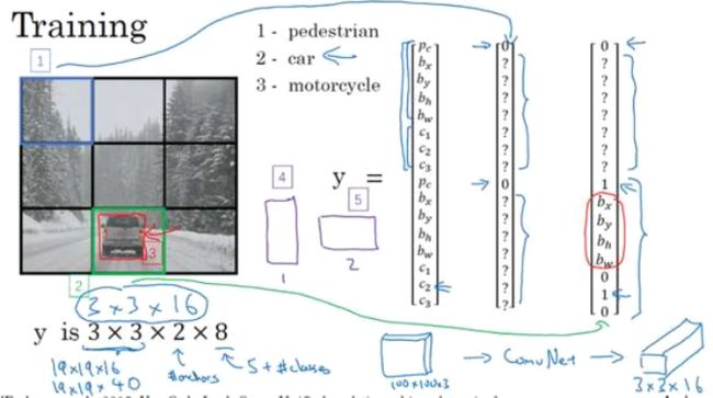
YOLO算法

paper：You Only Look Once：Unified real-time object detection（难度高）

IOU（intersection over union）交并比

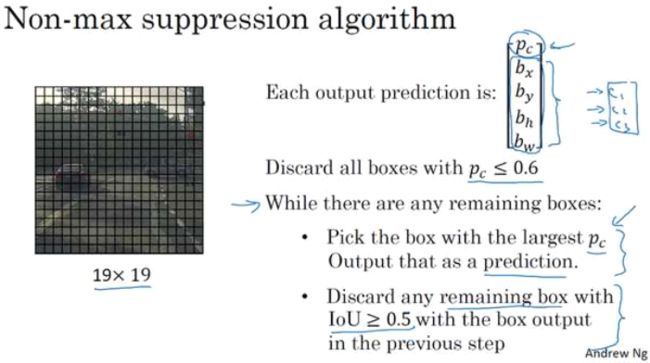
Non-max suppression

Anchor box：检测一个格子内多目标

propose region（候选区域）

Yolo实现代码

def yolo_filter_boxes(box_confidence, boxes, box_class_probs, threshold = .6):
    """Filters YOLO boxes by thresholding on object and class confidence.
    
    Arguments:
    box_confidence -- tensor of shape (19, 19, 5, 1)
    boxes -- tensor of shape (19, 19, 5, 4)
    box_class_probs -- tensor of shape (19, 19, 5, 80)
    threshold -- real value, if [ highest class probability score < threshold], then get rid of the corresponding box
    
    Returns:
    scores -- tensor of shape (None,), containing the class probability score for selected boxes
    boxes -- tensor of shape (None, 4), containing (b_x, b_y, b_h, b_w) coordinates of selected boxes
    classes -- tensor of shape (None,), containing the index of the class detected by the selected boxes
    
    Note: "None" is here because you don't know the exact number of selected boxes, as it depends on the threshold. 
    For example, the actual output size of scores would be (10,) if there are 10 boxes.
    """
    
    # Step 1: Compute box scores
    
    scores = box_confidence * box_class_probs # 每个cell里的各种分类的概率
    

    # Step 2: Find the box_classes thanks to the max box_scores, keep track of the corresponding score
    
    index = K.argmax(scores, axis = -1)    # 维度在倒数第一各种分类概率里的最大值的索引
    box_class_scores = K.max(index, axis = -1, keepdims = False) # 5个anchor中值最大的cell值
    
    
    
    # Step 3: Create a filtering mask based on "box_class_scores" by using "threshold". The mask should have the
    # same dimension as box_class_scores, and be True for the boxes you want to keep (with probability >= threshold)
    
    
    mask = box_class_scores >= threshold
    
    ### END CODE HERE ###
    
    # Step 4: Apply the mask to scores, boxes and classes
    
    scores = tf.boolean_mask(box_class_scores, mask)
    boxes = tf.boolean_mask(boxes, mask)
    classes = tf.boolean_mask(box_classes, mask）
    
    return scores, boxes, classes
                              
                              
                              
                              
                              
                              
                              
                              
                              
                              
                              
 # 交并比
 def iou(box1, box2):
    """Implement the intersection over union (IoU) between box1 and box2
    # 左下 右上
    Arguments:
    box1 -- first box, list object with coordinates (x1, y1, x2, y2)
    box2 -- second box, list object with coordinates (x1, y1, x2, y2)
    """

    # Calculate the (y1, x1, y2, x2) coordinates of the intersection of box1 and box2. Calculate its Area.
    ### START CODE HERE ### (≈ 5 lines)
    xi1 = max(box1[0], box2[0])
    yi1 = max(box1[1], box2[1])
    xi2 = min(box1[2], box2[2])
    yi2 = min(box1[3], box2[3])
    inter_area = (yi2 - yi1) * (xi2 - xi1)

    
    ### END CODE HERE ###    

    # Calculate the Union area by using Formula: Union(A,B) = A + B - Inter(A,B)
    ### START CODE HERE ### (≈ 3 lines)
    box1_area = (box1[3] - box1[1])*(box1[2] - box1[0]) 
    box2_area = (box2[3] - box2[1])*(box2[2] - box2[0])
    union_area = box1_area + box2_area - inter_area
    
    ### END CODE HERE ###
    
    # compute the IoU
    ### START CODE HERE ### (≈ 1 line)
    iou = inter_area / union_area
    ### END CODE HERE ###

    return iou
                              
    
                              
                              
                              
                              
                              
                              
                              
                              
 # 非最大值抑制
 
def yolo_non_max_suppression(scores, boxes, classes, max_boxes = 10, iou_threshold = 0.5):
    """
    Applies Non-max suppression (NMS) to set of boxes
    
    Arguments:
    scores -- tensor of shape (None,), output of yolo_filter_boxes()
    boxes -- tensor of shape (None, 4), output of yolo_filter_boxes() that have been scaled to the image size (see later)
    classes -- tensor of shape (None,), output of yolo_filter_boxes()
    max_boxes -- integer, maximum number of predicted boxes you'd like
    iou_threshold -- real value, "intersection over union" threshold used for NMS filtering
    
    Returns:
    scores -- tensor of shape (, None), predicted score for each box
    boxes -- tensor of shape (4, None), predicted box coordinates
    classes -- tensor of shape (, None), predicted class for each box
    
    Note: The "None" dimension of the output tensors has obviously to be less than max_boxes. Note also that this
    function will transpose the shapes of scores, boxes, classes. This is made for convenience.
    """
    
    max_boxes_tensor = K.variable(max_boxes, dtype='int32')     # tensor to be used in tf.image.non_max_suppression()
    K.get_session().run(tf.variables_initializer([max_boxes_tensor])) # initialize variable max_boxes_tensor
    
    # Use tf.image.non_max_suppression() to get the list of indices corresponding to boxes you keep
    ### START CODE HERE ### (≈ 1 line)
    
    index = tf.image.non_max_suppression(boxes,scores,max_boxes,iou_threshold=0.5)
    
    ### END CODE HERE ###
    
    # Use K.gather() to select only nms_indices from scores, boxes and classes
    ### START CODE HERE ### (≈ 3 lines)
    scores = tf.gather(scores,index,axis=0)
    boxes = tf.gather(boxes, index, axis = 0)
    classes = tf.gather(classes, index, axis = 0)
    ### END CODE HERE ###
    
    return scores, boxes, classes
                              
                              
                              
                              
                              
                              
 # 预测
 def yolo_eval(yolo_outputs, image_shape = (720., 1280.), max_boxes=10, score_threshold=.6, iou_threshold=.5):
    """
    Converts the output of YOLO encoding (a lot of boxes) to your predicted boxes along with their scores, box coordinates and classes.
    
    Arguments:
    yolo_outputs -- output of the encoding model (for image_shape of (608, 608, 3)), contains 4 tensors:
                    box_confidence: tensor of shape (None, 19, 19, 5, 1)
                    box_xy: tensor of shape (None, 19, 19, 5, 2)
                    box_wh: tensor of shape (None, 19, 19, 5, 2)
                    box_class_probs: tensor of shape (None, 19, 19, 5, 80)
    image_shape -- tensor of shape (2,) containing the input shape, in this notebook we use (608., 608.) (has to be float32 dtype)
    max_boxes -- integer, maximum number of predicted boxes you'd like
    score_threshold -- real value, if [ highest class probability score < threshold], then get rid of the corresponding box
    iou_threshold -- real value, "intersection over union" threshold used for NMS filtering
    
    Returns:
    scores -- tensor of shape (None, ), predicted score for each box
    boxes -- tensor of shape (None, 4), predicted box coordinates
    classes -- tensor of shape (None,), predicted class for each box
    """
    
    ### START CODE HERE ### 
    
    # Retrieve outputs of the YOLO model (≈1 line)
    box_confidence, box_xy, box_wh, box_class_probx = yolo_outputs

    # Convert boxes to be ready for filtering functions 
    boxes = yolo_boxes_to_corners(box_xy, box_wh) 

    # Use one of the functions you've implemented to perform Score-filtering with a threshold of score_threshold (≈1 line)
    scores, boxes, classes = yolo_filter_boxes(box_confidence, 
                                               boxes,box_class_probs, 
                                               score_threshold)

    # Scale boxes back to original image shape.
    boxes = scale_boxes(boxes, image_shape)

    # Use one of the functions you've implemented to perform Non-max suppression with a threshold of iou_threshold (≈1 line)
    scores, boxes, classes = yolo_non_max_suppression(scores, 
                                                      boxes, classes,
                                                      max_boxes, iou_threshold)
    
    ### END CODE HERE ###
    
    return scores, boxes, classes                             

脸部识别

Method

1. Given 3 image A, P, N：
   \[ L(A, P, N) = max(||f(A) - f(P)||^2\ - \ ||f(A) - f(N)||^2 \ + \alpha\ , 0 ) \]
   Training set: 10K pictures of 1k persons

   Paper:2015, FaceNet:A unified embedding for face recognition and clustering

2. Similarity function

   input
   \[ |f(x^{(i)})_k - f(x^{(j)})_k| \]
   create LS two classification ,one of the input uses percomputing

   paper:2014, DeepFace closing the gap to human level performance

Neural style transfer

paper:2015, A neural algorithm of artistic style

To run an image through this network, you just have to feed the image to the model. In TensorFlow, you can do so using the tf.assign function. In particular, you will use the assign function like this:

model["input"].assign(image)

This assigns the image as an input to the model. After this, if you want to access the activations of a particular layer, say layer 4_2 when the network is run on this image, you would run a TensorFlow session on the correct tensor conv4_2, as follows:

sess.run(model["conv4_2"])

1. Create an Interactive Session
2. Load the content image
3. Load the style image
4. Randomly initialize the image to be generated
5. Load the VGG16 model
6. Build the TensorFlow graph:
   • Run the content image through the VGG16 model and compute the content cost
   • Run the style image through the VGG16 model and compute the style cost
   • Compute the total cost
   • Define the optimizer and the learning rate
7. Initialize the TensorFlow graph and run it for a large number of iterations, updating the generated image at every step.

# Reset the graph
tf.reset_default_graph()

# Start interactive session
sess = tf.InteractiveSession()

import imageio
content_image = imageio.imread("images/louvre_small.jpg")
content_image = reshape_and_normalize_image(content_image)

style_image = imageio.imread("images/monet.jpg")
style_image = reshape_and_normalize_image(style_image)

generated_image = generate_noise_image(content_image)
imshow(generated_image[0])

5:load the VGG16 model

model = load_vgg_model("pretrained-model/imagenet-vgg-verydeep-19.mat")

6:omit some details

# Assign the content image to be the input of the VGG model.  
sess.run(model['input'].assign(content_image))

# Select the output tensor of layer conv4_2
out = model['conv4_2']

# Set a_C to be the hidden layer activation from the layer we have selected
a_C = sess.run(out)

# Set a_G to be the hidden layer activation from same layer. Here, a_G references model['conv4_2'] 
# and isn't evaluated yet. Later in the code, we'll assign the image G as the model input, so that
# when we run the session, this will be the activations drawn from the appropriate layer, with G as input.
a_G = out

# Compute the content cost
J_content = compute_content_cost(a_C, a_G)

def model_nn(sess, input_image, num_iterations = 200):
    
    # Initialize global variables (you need to run the session on the initializer)
    ### START CODE HERE ### (1 line)
    sess.run(tf.global_variables_initializer())
    ### END CODE HERE ###
    
    # Run the noisy input image (initial generated image) through the model. Use assign().
    ### START CODE HERE ### (1 line) 
    sess.run(model['input'].assign(input_image))
    ### END CODE HERE ###
    
    for i in range(num_iterations):
    
        # Run the session on the train_step to minimize the total cost
        ### START CODE HERE ### (1 line)
        sess.run(train_step)
        ### END CODE HERE ###
        
        # Compute the generated image by running the session on the current model['input']
        ### START CODE HERE ### (1 line)
        generated_image = sess.run(model['input'])
        ### END CODE HERE ###

        # Print every 20 iteration.
        if i%20 == 0:
            Jt, Jc, Js = sess.run([J, J_content, J_style])
            print("Iteration " + str(i) + " :")
            print("total cost = " + str(Jt))
            print("content cost = " + str(Jc))
            print("style cost = " + str(Js))
            
            # save current generated image in the "/output" directory
            save_image("output/" + str(i) + ".png", generated_image)
    
    # save last generated image
    save_image('output/generated_image.jpg', generated_image)
    
    return generated_image

序列模型

speech recognition, natural language process

music generation, Sentiment classification

DNA sequence analysis, Machine translation

Video activity recognition

RNN

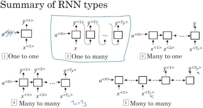
类型

GRU(gated recurrent units)门控循环单元

改变了RNN的隐藏层， 使其可以更好地捕捉深层连接，并改善了梯度消失问题，

Paper：（Chung J, Gulcehre C, Cho K H, et al. Empirical Evaluation of Gated Recurrent Neural
Networks on Sequence Modeling[J]. Eprint Arxiv, 2014.
Cho K, Merrienboer B V, Bahdanau D, et al. On the Properties of Neural Machine Translation:
Encoder-Decoder Approaches[J]. Computer Science, 2014.）

LSTM(Long short term memory)长短期记忆

Paper：（Hochreiter S, Schmidhuber J. Long Short-Term Memory[J]. Neural Computation, 1997,
9(8):1735-1780.）

NLP

use embedding

often used Cosine Similarity
\[ sim(e_w, e_{king} - e_{man} + e_{woman}) \]

\[ sim(u,v) = \frac {u^Tv} {||u||_2||v||_2} \]

or use (little)
\[ ||u-v||^2 \]

When you insert or overlay an "activate" clip, you will also update labels for ⟨⟩y⟨t⟩, so that 50 steps of the output now have target label 1