Gibbs采样

背景

之前介绍了Metropolis-Hastings采样算法，只考虑了一元概率分布的样本生成问题。本文讨论如何将MH算法扩展到多元分布上，重点讨论Gibbs采样算法。

Blockwise updating

Blockwise updating 是将MH扩展到多元分布上最简单的方法，就是选择一个和目标分布有相同维度的建议分布。例如如果要生成 N 元概率分布的样本，我们就采用一个 N 元的建议分布（proposal distribution）。在马尔可夫链状态转移过程中，接受或者拒绝整个建议（包含 N 个随机变量）。算法的流程如下所示：

1. 设置马尔可夫链的初始状态 X0=x⃗ 0

2. 对 t=0,1,2,3,… 循环进行以下过程

   (1) 第 t 时刻的马氏链的状态为 Xt=x⃗ t ，采样 y⃗ ∼q(y⃗ |x⃗ t)

   (2) 从均匀分布采样 u∼Uniform[0,1]

   (3) 如果 u<α(x⃗ t,y⃗ )=min[p(y⃗ )q(x⃗ t|y⃗ )p(x⃗ t)q(y⃗ |x⃗ t),1] ，则接受转移 x⃗ t→y⃗  ， Xt+1=y⃗ 

   (4) 否则不接受转移， Xt+1=x⃗ t

与之前MH算法的不同之处，就是将标量 x 替换成了 x⃗  。其中 x⃗ ={x1,x2,…,xN} 表示 N 维随机变量。

例子

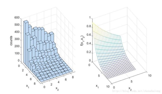
采用 Blockwise updating 方法对 Bivariate Exponential 分布进行采样。概率密度函数如下：

function y = bivexp(theta1,theta2)
%%返回Bivariate Exponential分布的概率密度函数
lambda1 = 0.5;
lambda2 = 0.1;
lambda = 0.01;
maxval = 8;
y = exp(-(lambda1+lambda)*theta1-(lambda2+lambda)*theta2-lambda*maxval);

采样过程代码如下：

%% Blockwise updating to sample from Bivariate Exponential

%% Initalize the MH sampler
T=10000; % Set the maximum number of iterations
x_min = [ 0 0 ]; % define minimum for theta1 and theta2
x_max = [ 8 8 ]; % define maximum for theta1 and theta2
seed=1; rand('state', seed ); randn('state',seed ); % set the random seed
x = zeros( 2 , T ); % Init storage space for our samples
% Use a uniform proposal distribution
x(1,1) = unifrnd( x_min(1) , x_max(1) ); % Start value for theta1
x(2,1) = unifrnd( x_min(2) , x_max(2) ); % Start value for theta2

%% Start sampling 
t=1;
while t < T % Iterate until we have T samples
    t = t + 1;
    % Propose a new value for theta
    y = unifrnd(thetamin,thetamax);
    pratio = bivexp(y(1),y(2))/bivexp(x(1,t-1),x(2,t-1));
    alpha = min([1,pratio]); % Calculate the acceptance ratio
    u = rand; % Draw a uniform deviate from [ 0 1 ]
    if u < alpha % Do we accept this proposal?
        x(:,t) = y; % proposal becomes new value for theta
    else
        x(:,t) = x(:,t-1); % copy old value of theta
    end
end

%% Display histogram of our samples
figure( 1 ); clf;
subplot( 1,2,1 );
nbins = 10;
xbins1 = linspace( x_min(1) , x_max(1) , nbins );
xbins2 = linspace( x_min(2) , x_max(2) , nbins );
hist3( x' , 'Edges' , {xbins1 xbins2} );
xlabel( 'x_1' ); ylabel('x_2' ); zlabel( 'counts' );
az = 61; el = 30;
view(az, el);

%% Plot the theoretical density
subplot(1,2,2);
nbins = 20;
xbins1 = linspace( x_min(1) , x_max(1) , nbins );
xbins2 = linspace( x_min(2) , x_max(2) , nbins );
[ x1grid , x2grid ] = meshgrid( xbins1 , xbins2 );
ygrid = bivexp( x1grid , x2grid );
mesh( x1grid , x2grid , ygrid );
xlabel( 'x_1' ); ylabel('x_2' );
zlabel( 'f(x_1,x_2)' );
view(az, el);

实验结果如下：

Componentwise updating

MH算法中，选择合适的建议分布是比较困难的，对于高维分布更是如此。前面介绍的 Blockwise updating的方法，拒绝率往往很高，导致算法的效率不高。下面介绍一种与之相对应的采样方法：Componentwise updating。与 Blockwise 提出包含 N 个元素的建议然后接受或拒绝整个建议 y⃗  不同，Componentwise 每次针对 xt 的第 i 个元素提出建议 yi ，然后接受或拒绝这个建议。

例如对于一个随机变量 x⃗ =(x1,x2) 的二维分布进行采样。我们首先设置初始状态 x⃗ (0)=(x(0)1,x(0)2) 。在第 t 次迭代，我们针对随机变量 x⃗  的第一个维度，首先根据 x(t−1)1 提出建议 x∗1 ，然后计算由状态 (xt−11,xt−12) 转移到状态 (x∗1,xt−12) 的接受率，根据接受率决定是否接受建议 x∗1 。在上面这个过程中我们只改变了第一维的元素，而第二维的元素保持不变。与之类似我们针对岁间变量 x⃗  的第二个维度，首先根据 x(t−1)2 提出建议 x∗2 ，然后计算由状态 (xt1,xt−12) 转移到状态 (xt1,x∗2) 的接受率，根据接受率决定是否接受建议 x∗2 。在上面这个过程中我们只改变了第二维的元素，而第一维的元素保持不变。算法流程如下：

1. 设置马尔可夫链的初始状态 x⃗ (0)
2. 对 t=0,1,2,3,… 循环进行以下过程
   第 t 时刻的马氏链的状态为 x⃗ (t)=(x(t)1,x(t)2,…,x(t)n) ，对 i=1,2,3,…,n 循环进行以下过程
   （1）采样 x∗i∼q(x∗i|x(t)i)
   （2）从均匀分布采样 u∼Uniform[0,1]
   （3）如果 u<min[p(x(t+1)1,x(t+1)2,…,x(t+1)i−1,x∗i,x(t)i+1,…,x(t)n)q(x(t)i|x∗i)p(x(t+1)1,x(t+1)2,…,x(t+1)i−1,x(t)i,x(t)i+1,…,x(t)n)q(x∗i|x(t)i),1] ，则接受转移 x(t)i→x∗i , xt+1i=x∗i ；否则拒绝转移， xt+1i=x(t)i

注：由于每次只改变随机变量一个维度的值，而其他维度的值保持不变。对于 n 维随机变量，建议分布为 n 维分布：

q((x(t−1)1,x(t−1)2,…,x∗i,…,x(t−1)n)|(x(t−1)1,x(t−1)2,…,x(t−1)i,…,x(t−1)n))

Componentwise updating其实是对上式做了一个限制，将其简化为一个一维分布：

q(x∗i|x(t−1)i)

例子

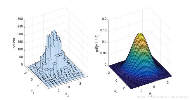
采用 Componentwise updating 方法对二维正态分布进行采样。概率密度函数如下：

12π|Σ|1/2exp{−12(x⃗ −u⃗ )TΣ−1(x⃗ −u⃗ )}

其中，

u⃗ =[0,0]

Σ=[10.30.31]

采用的建议分布为正太分布， σ=1 。
实验代码如下：

%% Component?wise updating. Use a normal proposal distribution
%Parameters of the Bivariate normal
mu = [0,0];
sigma = [1,0.3;0.3,1];

%% Initialize the Metropolis sampler
T = 5000; % Set the maximum number of iterations
propsigma = 1; % standard dev. of proposal distribution
thetamin = [-3,-3]; % define minimum for theta1 and theta2
thetamax = [3,3]; % define maximum for theta1 and theta2
seed=1; rand( 'state', seed ); randn('state',seed ); % set the random seed
state = zeros( 2 , T ); % Init storage space for the state of the sampler
theta1 = unifrnd( thetamin(1) , thetamax(1) ); % Start value for theta1
theta2 = unifrnd( thetamin(2) , thetamax(2) ); % Start value for theta2
t = 1; % initialize iteration at 1
state(1,t) = theta1; % save the current state
state(2,t) = theta2;

%% Start sampling
while t < T % Iterate until we have T samples
    t = t + 1;

    %% Propose a new value for theta1
    new_theta1 = normrnd( theta1 , propsigma );
    pratio = mvnpdf( [ new_theta1 theta2 ] , mu , sigma ) / mvnpdf( [ theta1 theta2 ] , mu , sigma );
    alpha = min( [ 1 pratio ] ); % Calculate the acceptance ratio
    u = rand; % Draw a uniform deviate from [ 0 1 ]
    if u < alpha % Do we accept this proposal?
        theta1 = new_theta1; % proposal becomes new value for theta1
    end

    %% Propose a new value for theta2
    new_theta2 = normrnd( theta2 , propsigma );
    pratio = mvnpdf( [ theta1 new_theta2 ] , mu , sigma ) / mvnpdf( [ theta1 theta2 ] , mu , sigma );
    alpha = min( [ 1 pratio ] ); % Calculate the acceptance ratio
    u = rand; % Draw a uniform deviate from [ 0 1 ]
    if u < alpha % Do we accept this proposal?
        theta2 = new_theta2; % proposal becomes new value for theta2
    end

    %% Save state
    state(1,t) = theta1;
    state(2,t) = theta2;
end

%% Display histogram of our samples
figure( 1 ); clf;
subplot( 1,2,1 );
nbins = 12;
thetabins1 = linspace( thetamin(1) , thetamax(1) , nbins );
thetabins2 = linspace( thetamin(2) , thetamax(2) , nbins );
hist3( state' , 'Edges' , {thetabins1 thetabins2} );
xlabel( '\theta 1' ); ylabel('\theta 2' ); zlabel( 'counts' );
az = 61; el = 30; view(az, el);

%% Plot the theoretical density
subplot(1,2,2);
nbins = 50;
thetabins1 = linspace( thetamin(1) , thetamax(1) , nbins );
thetabins2 = linspace( thetamin(2) , thetamax(2) , nbins );
[ theta1grid , theta2grid ] = meshgrid( thetabins1 , thetabins2 );
zgrid = mvnpdf( [ theta1grid(:) theta2grid(:)] , mu , sigma );
zgrid = reshape( zgrid , nbins , nbins );
surf( theta1grid , theta2grid , zgrid );
xlabel( '\theta 1' ); ylabel('\theta 2' );
zlabel( 'pdf(\theta 1,\theta 2)' );
view(az, el);
xlim([thetamin(1) thetamax(1)]); ylim([thetamin(2) thetamax(2)]);

实验结果：

注：对未归一化的概率分布 p(x⃗ )=p~(x⃗ )Xp Blockwise updating 和 Componentwise updating 采样算法仍然适用。只需把接受率 α 中的 p(∗) 变为 p~(∗) ，与归一化常数 Xp 无关！

Gibbs 采样

拒绝采样和MH 采样算法难以选择合适的建议分布，尤其是在高维的情况下。另外当接受率较低时，大量的样本被拒绝，导致算法效率不高。Gibbs 采样算法，不需要指定建议分布，而且所有的样本都被接受，因而是一种更有效的算法。但是，Gibbs 采样只适用于条件分布已知的情况。

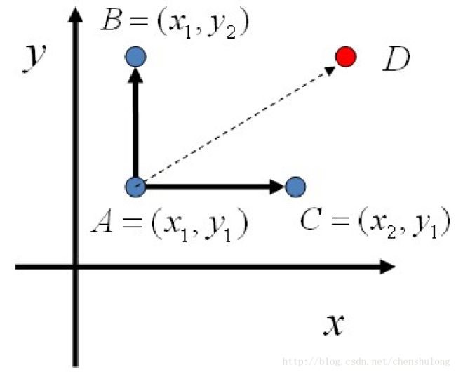
我们以二维分布为例来说明 Gibbs 采样过程。假设有一个二维分布 p(x,y) ，考察 x 轴坐标相同的两个点 A(x1,y1) 和 B(x1,y2)

我们发现

p(x1,y1)p(y2|x1)=p(x1)p(y1|x1)p(y2|x1)

p(x1,y2)p(y1|x1)=p(x1)p(y2|x1)p(y1|x1)

所以得到：

p(x1,y1)p(y2|x1)=p(x1,y2)p(y1|x1)

即

p(A)p(y2|x1)=p(B)p(y1|x1)

基于以上等式，我们发现，在 x=x1 这条平行于 y 轴的直线上，如果使用条件分布 p(y|x1) 作为任何两点之间的转移概率（ 接受率为1），那么 p(x,y) 满足细致平稳条件，恰好是该马尔可夫链的稳态分布。
同样的，如果我们在 y=y1 这条直线上任取亮点 A(x1,y1) 和 C(x2,y1) ，也有如下等式成立：

p(A)p(x2|y1)=p(C)p(x1|y1)

于是我们可以如下构造平面上任意两点之间的状态转移矩阵 Q ：

Q(A→B)Q(A→C)Q(A→D)=p(yB|x1) =p(xC|y1) =0 如果xA=xB=x1如果yA=yC=y1其它

有了如上的转移矩阵 Q ，我们很容易验证对平面上任意两点 X,Y ，满足细致平稳条件：

p(X)p(X→Y)=p(Y)Q(Y→X)

于是这个二维空间上的马氏链将收敛到平稳分布 p(x,y) 。这个算法就是 Gibbs Sampling 算法，是 Stuart Geman 和 Donald Geman 这两兄弟于1984年提出的。之所以叫做 Gibbs 采样，是因为他们研究了 Gibbs random field，这个算法在现代贝叶斯分析中占据重要位置。

二维 Gibbs 采样算法流程如下所示：

MCMC的采样过程如下图所示：

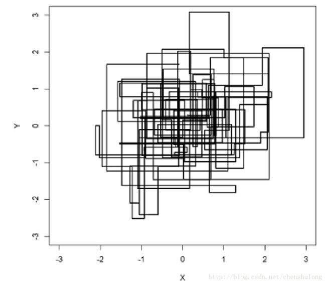
可以发现在采样过程中，马氏链的转移只是轮换地沿着坐标轴 x 轴 和 y 轴做转移，于是得到样本 (x0,y0),(x0,y1),(x1,y1),(x1,y2),(x2,y2),… 马氏链收敛后，最终得到的样本就是分布 p(x,y) 的样本，而收敛之前的阶段称之为 burn-in period。

注：大部分资料中的 Gibbs 算法都是坐标轴轮换采样的，但是这其实这不是必须的。最一般的情况可以是，在第 t 次迭代中，可以在 x 轴和 y 轴之间随机选择一个坐标轴，然后按条件概率做转移，马氏链也是一样收敛的。轮换两个坐标轴只是一种方便的形式。

下面我们将Gibbs 采样推广到 n 维的情况，细致平稳条件仍然成立：

p(x1,x2,…,xj,…,xn)p(x′j|x1,x2,…,xj−1,xj+1,…,xn)=p(x1,x2,…,x′j,…,xn)p(xj|x1,x2,…,xj−1,xj+1,…,xn)

容易验证对所有的坐标轴 i=1,2,…,n 上式均成立。所以 n 维空间中对于概率分布 p(x1,x2,…,xn) 可以如下定义状态转移矩阵：

1. 如果当前状态为 (x1,x2,…,xj,…,xn) ，马氏链转移过程中只能沿着坐标轴转移。若沿着第 j 个坐标轴转移，转移到状态 (x1,x2,…,x′j,…,xn) 的概率由条件概率 p(x′j|x1,x2,…,xj−1,xj+1,…,xn) 定义
2. 其它无法沿着单个坐标轴进行的转移，转移概率均设置为0

n 维情况下，Gibbs采样过程如下所示：

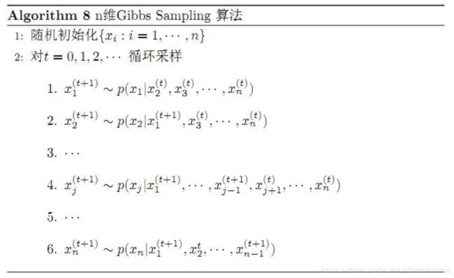
以上算法收敛后，得到的就是概率分布 p(x1,x2,…,xn) 的样本，当然这些样本并不独立，但是我们此处只要求采样得到的样本符合制定的概率分布，并不要求独立。同样的，在以上算法中，坐标轴的轮换也不是必须的，可以在坐标轴轮换中引入随机性，这时候转移矩阵 Q 中任何两个点的转移概率就会包含坐标轴选择的概率而在通常的 Gibbs 采样算法中，坐标轴轮换是一个确定性的过程，也就是在一次迭代中，沿着某个坐标轴转移的概率是1。