基于tensorflow_gpu 1.9.0实现的第三个神经网络：对波士顿的房价预测（回归问题）

示例来源于Tensorflow的官方教程。
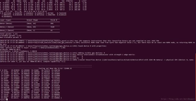
基于tensorflow_gpu 1.9.0实现的第三个神经网络：对波士顿的房价预测（回归问题），代码如下：

#!/usr/bin/env python
from __future__ import print_function
import tensorflow as tf
from tensorflow import keras
import numpy as np
import pandas as pd
import matplotlib.pyplot as plt

print(tf.__version__)

boston_housing = keras.datasets.boston_housing
(train_data, train_labels), (test_data, test_labels) = boston_housing.load_data()

# Shuffle the training set
order = np.argsort(np.random.random(train_labels.shape))
train_data = train_data[order]
train_labels = train_labels[order]

# The dataset contains 13 different features:
#   Per capita crime rate.
#   The proportion of residential land zoned for lots over 25,000 square feet.
#   The proportion of non-retail business acres per town.
#   Charles River dummy variable (= 1 if tract bounds river; 0 otherwise).
#   Nitric oxides concentration (parts per 10 million).
#   The average number of rooms per dwelling.
#   The proportion of owner-occupied units built before 1940.
#   Weighted distances to five Boston employment centers.
#   Index of accessibility to radial highways.
#   Full-value property-tax rate per $10,000.
#   Pupil-teacher ratio by town.
#   1000 * (Bk - 0.63) ** 2 where Bk is the proportion of Black people by town.
#   Percentage lower status of the population.
# Each one of these input data features is stored using a different scale. Some
# features are represented by a proportion between 0 and 1, other features are
# ranges between 1 and 12, some are ranges between 0 and 100, and so on. This is
# often the case with real-world data, and understanding how to explore and
# clean such data is an important skill to develop.
print("Training set: {}".format(train_data.shape))  # 404 examples, 13 features
print("Testing set: {}".format(test_data.shape))  # 102 examples, 13 features
print(train_data[0])

column_names = ['CRIM', 'ZN', 'INDUS', 'CHAS', 'NOX', 'RM', 'AGE', 'DIS', 'RAD',
                'TAX', 'PTRATIO', 'B', 'LSTAT']
df = pd.DataFrame(train_data, columns=column_names)
print(df.head())

print(train_labels[0:10])  # Display first 10 entries.

# Normalize features

# Test data is *not* used when calculating the mean and std.
mean = train_data.mean(axis=0)
std = train_data.std(axis=0)
train_data = (train_data - mean) / std
test_data = (test_data - mean) / std

print(train_data[0])  # First training sample, normalized.

# Create the model


def build_model():
    model = keras.Sequential([
        keras.layers.Dense(64, activation=tf.nn.relu,
                           input_shape=(train_data.shape[1], )),
        keras.layers.Dense(64, activation=tf.nn.relu),
        keras.layers.Dense(1)
    ])

    optimizer = tf.train.RMSPropOptimizer(0.001)
    model.compile(loss='mse', optimizer=optimizer, metrics=['mae'])
    return model


model = build_model()
model.summary()

# Train the model

# Display training progress by printing a single dot for each completed epoch.


class PrintDot(keras.callbacks.Callback):
    def on_epoch_end(self, epoch, logs):
        if epoch % 100 == 0:
            print('')
        print('.', end='')


# The patience parameter is the amount of epochs to check for improvement.
early_stop = keras.callbacks.EarlyStopping(monitor='val_loss', patience=20)

EPOCHS = 500
# Store training stats

history = model.fit(train_data, train_labels, epochs=EPOCHS,
                    validation_split=0.2, verbose=0,
                    callbacks=[early_stop, PrintDot()])

# Evaluate the model
[loss, mae] = model.evaluate(test_data, test_labels, verbose=0)
print("Testing set Mean Abs Error: ${:7.2f}".format(mae * 1000))

# Predict
test_predictions = model.predict(test_data).flatten()
print(test_predictions)

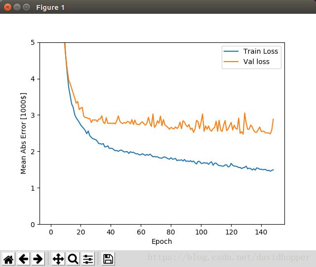
def plot_history(history):
    plt.figure()
    plt.xlabel('Epoch')
    plt.ylabel('Mean Abs Error [1000$]')
    plt.plot(history.epoch, np.array(history.history['mean_absolute_error']),
             label='Train Loss')
    plt.plot(history.epoch, np.array(history.history['val_mean_absolute_error']),
             label='Val loss')
    plt.legend()
    plt.ylim([0, 5])
    plt.show()

plot_history(history)

运行该程序之前，需要先根据我的另一篇博客《Ubuntu 16.04安装tensorflow_gpu 1.9.0的方法》，安装tensorflow_gpu 1.9.0，然后安装numpy、pandas、matplotlib等工具包，此外还需要安装python-tk，命令如下：

sudo pip install numpy
sudo pip install pandas
sudo pip install matplotlib
sudo apt-get install python-tk

运行结果如下：