数据挖掘实战（一）

这是做Kaggle的一个比赛的初步探索https://www.kaggle.com/c/reducing-commercial-aviation-fatalities

主要包括数据预处理、探索性分析、特征工程和建模四个步骤

1.数据预处理：

import warnings
import itertools
import numpy as np 
import pandas as pd
import seaborn as sns
import lightgbm as lgb
import matplotlib.pyplot as plt
from tqdm import tqdm_notebook as tqdm
from sklearn.preprocessing import MinMaxScaler
from sklearn.model_selection import train_test_split
from sklearn.metrics import confusion_matrix, log_loss

warnings.simplefilter(action='ignore')
sns.set_style('whitegrid')

读取数据和查看数据基本情况：

dtypes = {"crew": "int8",
          "experiment": "category",
          "time": "float32",
          "seat": "int8",
          "eeg_fp1": "float32",
          "eeg_f7": "float32",
          "eeg_f8": "float32",
          "eeg_t4": "float32",
          "eeg_t6": "float32",
          "eeg_t5": "float32",
          "eeg_t3": "float32",
          "eeg_fp2": "float32",
          "eeg_o1": "float32",
          "eeg_p3": "float32",
          "eeg_pz": "float32",
          "eeg_f3": "float32",
          "eeg_fz": "float32",
          "eeg_f4": "float32",
          "eeg_c4": "float32",
          "eeg_p4": "float32",
          "eeg_poz": "float32",
          "eeg_c3": "float32",
          "eeg_cz": "float32",
          "eeg_o2": "float32",
          "ecg": "float32",
          "r": "float32",
          "gsr": "float32",
          "event": "category",
         }

train_df = pd.read_csv("J:/CommercialAviationFatality/train.csv", dtype=dtypes)
test_df = pd.read_csv("J:/CommercialAviationFatality/test.csv", dtype=dtypes)
train_df.info()
train_df.head()
test_df.head()

 探索性数据分析

plt.figure(figsize=(15,10))
sns.countplot(train_df['event'])
plt.xlabel("State of the pilot", fontsize=12)
plt.ylabel("Count", fontsize=12)
plt.title("Target repartition", fontsize=15)
plt.show()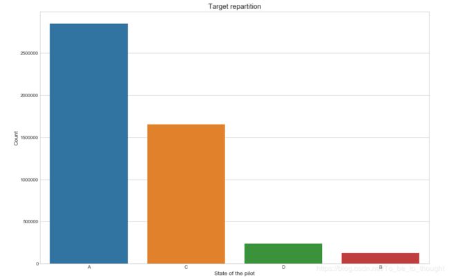

plt.figure(figsize=(15,10))
sns.countplot('experiment', hue='event', data=train_df)
plt.xlabel("Experiment and state of the pilot", fontsize=12)
plt.ylabel("Count (log)", fontsize=12)
plt.yscale('log')
plt.title("Target repartition for different experiments", fontsize=15)
plt.show()

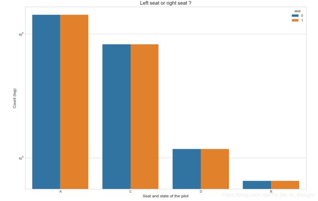
plt.figure(figsize=(15,10))
sns.countplot('event', hue='seat', data=train_df)
plt.xlabel("Seat and state of the pilot", fontsize=12)
plt.ylabel("Count (log)", fontsize=12)
plt.yscale('log')
plt.title("Left seat or right seat ?", fontsize=15)
plt.show()

 

plt.figure(figsize=(15,10))
sns.violinplot(x='event', y='time', data=train_df.sample(50000))
plt.ylabel("Time (s)", fontsize=12)
plt.xlabel("Event", fontsize=12)
plt.title("Which time do events occur at ?", fontsize=15)
plt.show()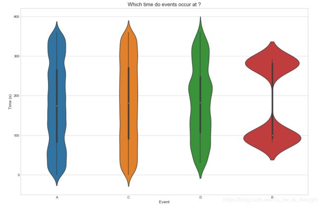

plt.figure(figsize=(15,10))
sns.distplot(test_df['time'], label='Test set')
sns.distplot(train_df['time'], label='Train set')
plt.legend()
plt.xlabel("Time (s)", fontsize=12)
plt.title("Reparition of the time feature", fontsize=15)
plt.show()

eeg_features = ["eeg_fp1", "eeg_f7", "eeg_f8", "eeg_t4", "eeg_t6", "eeg_t5", "eeg_t3", "eeg_fp2", "eeg_o1", "eeg_p3", "eeg_pz", "eeg_f3", "eeg_fz", "eeg_f4", "eeg_c4", "eeg_p4", "eeg_poz", "eeg_c3", "eeg_cz", "eeg_o2"]
plt.figure(figsize=(20,25))
i = 0

for egg in eeg_features:
    i += 1
    plt.subplot(5, 4, i)
    sns.boxplot(x='event', y=egg, data=train_df.sample(50000), showfliers=False)

plt.show()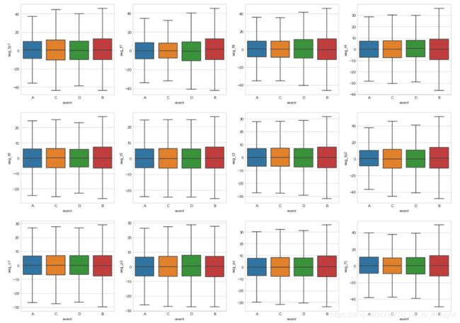

plt.figure(figsize=(20,25))
plt.title('Eeg features distributions')
i = 0

for eeg in eeg_features:
    i += 1
    plt.subplot(5, 4, i)
    sns.distplot(test_df.sample(10000)[eeg], label='Test set', hist=False)
    sns.distplot(train_df.sample(10000)[eeg], label='Train set', hist=False)
    plt.xlim((-500, 500))
    plt.legend()
    plt.xlabel(eeg, fontsize=12)

plt.show()

plt.figure(figsize=(15,10))
sns.violinplot(x='event', y='ecg', data=train_df.sample(50000))
plt.ylabel("Electrocardiogram Signal (µV)", fontsize=12)
plt.xlabel("Event", fontsize=12)
plt.title("Electrocardiogram signal influence", fontsize=15)
plt.show()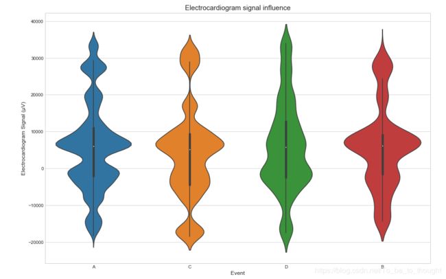

plt.figure(figsize=(15,10))
sns.distplot(test_df['ecg'], label='Test set')
sns.distplot(train_df['ecg'], label='Train set')
plt.legend()
plt.xlabel("Electrocardiogram Signal (µV)", fontsize=12)
plt.title("Electrocardiogram Signal Distribution", fontsize=15)
plt.show()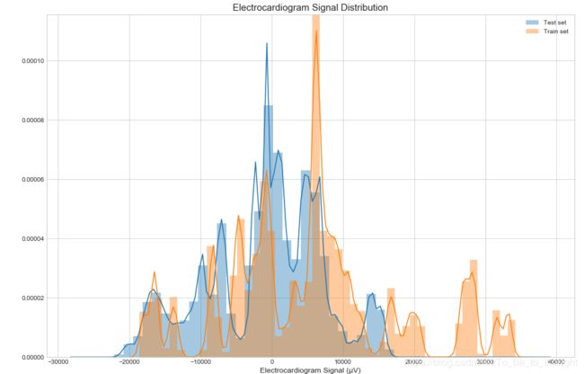

plt.figure(figsize=(15,10))
sns.violinplot(x='event', y='r', data=train_df.sample(50000))
plt.ylabel("Respiration Signal (µV)", fontsize=12)
plt.xlabel("Event", fontsize=12)
plt.title("Respiration influence", fontsize=15)
plt.show()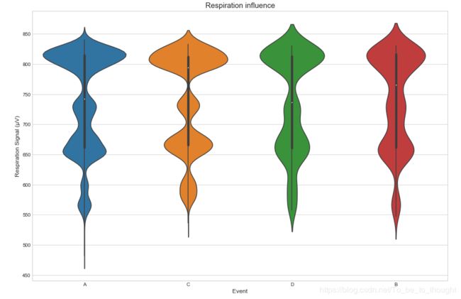

plt.figure(figsize=(15,10))
sns.distplot(test_df['r'], label='Test set')
sns.distplot(train_df['r'], label='Train set')
plt.legend()
plt.xlabel("Respiration Signal (µV)", fontsize=12)
plt.title("Respiration Signal Distribution", fontsize=15)
plt.show()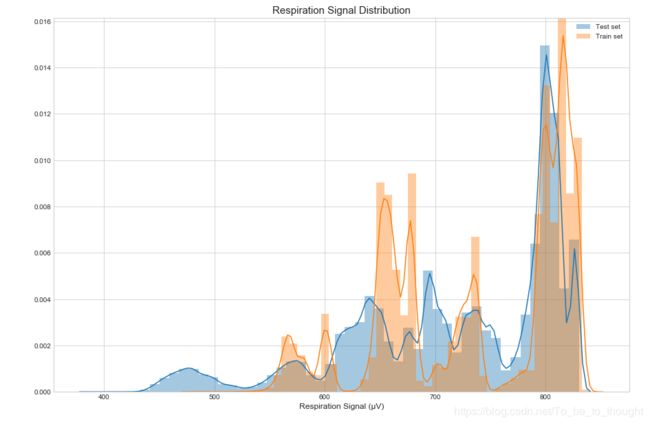

plt.figure(figsize=(15,10))
sns.violinplot(x='event', y='gsr', data=train_df.sample(50000))
plt.ylabel("Electrodermal activity measure (µV)", fontsize=12)
plt.xlabel("Event", fontsize=12)
plt.title("Electrodermal activity influence", fontsize=15)
plt.show()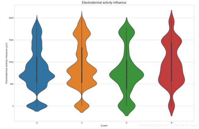

plt.figure(figsize=(15,10))
sns.distplot(test_df['gsr'], label='Test set')
sns.distplot(train_df['gsr'], label='Train set')
plt.legend()
plt.xlabel("Electrodermal activity measure (µV)", fontsize=12)
plt.title("Electrodermal activity Distribution", fontsize=15)
plt.show()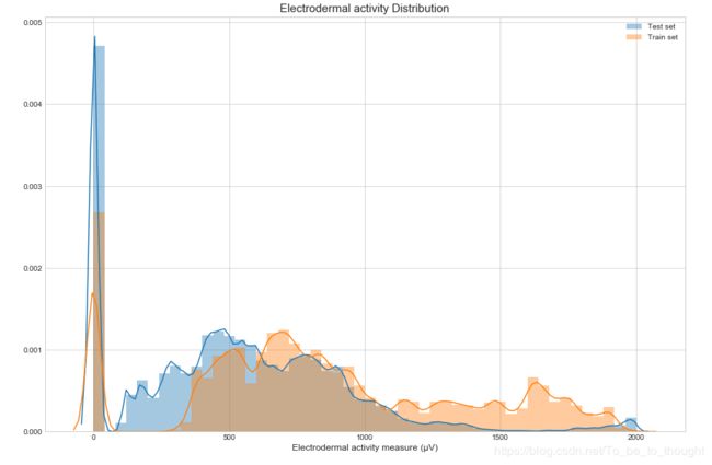

features_n = ["eeg_fp1", "eeg_f7", "eeg_f8", "eeg_t4", "eeg_t6", "eeg_t5", "eeg_t3", "eeg_fp2", "eeg_o1", "eeg_p3", "eeg_pz", "eeg_f3", "eeg_fz", "eeg_f4", "eeg_c4", "eeg_p4", "eeg_poz", "eeg_c3", "eeg_cz", "eeg_o2", "ecg", "r", "gsr"]
train_df['pilot'] = 100 * train_df['seat'] + train_df['crew']
test_df['pilot'] = 100 * test_df['seat'] + test_df['crew']

print("Number of pilots : ", len(train_df['pilot'].unique()))

def normalize_by_pilots(df):
    pilots = df["pilot"].unique()
    for pilot in tqdm(pilots):
        ids = df[df["pilot"] == pilot].index
        scaler = MinMaxScaler()
        df.loc[ids, features_n] = scaler.fit_transform(df.loc[ids, features_n])
        
    return df

train_df = normalize_by_pilots(train_df)
test_df = normalize_by_pilots(test_df)


train_df, val_df = train_test_split(train_df, test_size=0.2, random_state=420)
print(f"Training on {train_df.shape[0]} samples.")

features = ["crew", "seat"] + features_n
      
def run_lgb(df_train, df_test):
    # Classes as integers
    dic = {'A': 0, 'B': 1, 'C': 2, 'D': 3}
    try:
        df_train["event"] = df_train["event"].apply(lambda x: dic[x])
        df_test["event"] = df_test["event"].apply(lambda x: dic[x])
    except: 
        pass
    
    params = {"objective" : "multiclass",
              "num_class": 4,
              "metric" : "multi_error",
              "num_leaves" : 30,
              "min_child_weight" : 50,
              "learning_rate" : 0.1,
              "bagging_fraction" : 0.7,
              "feature_fraction" : 0.7,
              "bagging_seed" : 420,
              "verbosity" : -1
             }
    
    lg_train = lgb.Dataset(df_train[features], label=(df_train["event"]))
    lg_test = lgb.Dataset(df_test[features], label=(df_test["event"]))
    model = lgb.train(params, lg_train, 1000, valid_sets=[lg_test], early_stopping_rounds=50, verbose_eval=100)
    
    return model


model = run_lgb(train_df, val_df)
fig, ax = plt.subplots(figsize=(12,10))
lgb.plot_importance(model, height=0.8, ax=ax)
ax.grid(False)
plt.ylabel('Feature', size=12)
plt.xlabel('Importance', size=12)
plt.title("Importance of the Features of our LightGBM Model", fontsize=15)
plt.show()


pred_val = model.predict(val_df[features], num_iteration=model.best_iteration)
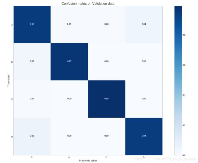
print("Log loss on validation data :", round(log_loss(np.array(val_df["event"].values), pred_val), 3))

def plot_confusion_matrix(cm, classes, title='Confusion matrix', normalize=False, cmap=plt.cm.Blues):
    if normalize:
        cm = cm.astype('float') / cm.sum(axis=1)[:, np.newaxis]
    fmt = '.2f' if normalize else 'd'

    fig, ax = plt.subplots(figsize=(15, 10))
    ax.imshow(cm, interpolation='nearest', cmap=cmap)

    plt.imshow(cm, interpolation='nearest', cmap=cmap)
    plt.title(title, size=15)
    plt.colorbar()
    plt.grid(False)
    tick_marks = np.arange(len(classes))
    plt.xticks(tick_marks, classes, rotation=45)
    plt.yticks(tick_marks, classes)

    thresh = (cm.max()+cm.min()) / 2.
    for i, j in itertools.product(range(cm.shape[0]), range(cm.shape[1])):
        plt.text(j, i, format(cm[i, j], fmt),
                 horizontalalignment="center",
                 color="white" if cm[i, j] > thresh else "black")

    plt.tight_layout()
    plt.ylabel('True label', size=12)
    plt.xlabel('Predicted label', size=12)

conf_mat_val = confusion_matrix(np.argmax(pred_val, axis=1), val_df["event"].values)
plot_confusion_matrix(conf_mat_val, ["A", "B", "C", "D"], title='Confusion matrix on Validation data', normalize=True)