多变量线性回归（一）

搭建编程环境

此处推荐安装Octave，如若已安装Matlab也可。这里不过多叙述如何安装Octave或Matlab，请自行查阅相关资料。

多维特征（Multiple Features）

之前我们学习了单变量线性回归，现在我们继续利用房价的例子来学习多变量线性回归。

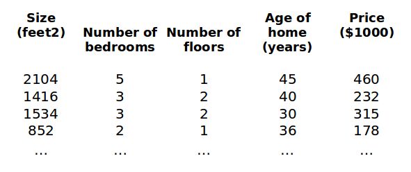
如上图所示，我们对房价模型增加一些特征，例如：房间的数量、楼层数和房屋使用年限。对此，我们分别令x₁，x₂，x₃和x₄表示房屋面积、房间的数量、楼层数和房屋使用年限。

这里增添了一些特征，我们也要引入一系列新的符号标记：

• n：代表特征的数量
• x⁽ⁱ⁾：代表第i个训练示例，即表示特征矩阵中的第i行
• x_j⁽ⁱ⁾：代表特征矩阵中第i行的第j个特征

因此，我们的多变量线性回归的表达式为：
　　h_θ(x) = θ₀+θ₁x₁+θ₂x₂+···+θ_nx_n

这个公式中有n+1个参数和n个变量，为了简化该公式，我们引入x₀=1（x₀⁽ⁱ⁾=1），则公式可以转化为：
　　h_θ(x) = θ₀x₀+θ₁x₁+θ₂x₂+···+θ_nx_n

此时公式中有n+1个参数和n+1个变量，此时我们可以将参数和变量看成n+1维的向量（即θ表示n+1维的（参数）向量，X表示n+1维的（变量）向量），则我们可将公式简化成：
　　h_θ(x) = θ^TX

补充笔记

Multiple Features

Linear regression with multiple variables is also known as "multivariate linear regression".

We now introduce notation for equations where we can have any number of input variables.

• x_j⁽ⁱ⁾ = value of feature j in the i^th training example
• x⁽ⁱ⁾ = the input (features) of the i^th training example

Note:

• m = the number of training example
• n = the number of features

The multivariable form of the hypothesis function accommodating these multiple features is as follows:
　　h_θ(x) = θ₀+θ₁x₁+θ₂x₂+···+θ_nx_n

In order to develop intuition about this function, we can think about θ₀ as the basic price of a house, θ₁ as the price per square meter, θ₂ as the price per floor, etc. x₁ will be the number of square meters in the house, x₂ the number of floors, etc.

Using the definition of matrix multiplication, our multivariable hypothesis function can be concisely represented as:

This is a vectorization of our hypothesis function for one training example.

多变量梯度下降（Gradient Descent For Multiple Variables）

与之前的单变量线性回归类似，我们也构建了一个代价函数J：

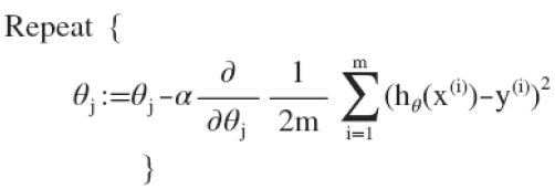
我们的目标与在单变量线性回归中一样，找出使得代价函数最小的一系列参数。在单变量线性回归中，我们引入梯度下降算法来找寻该参数。因此，在多变量线性回归中，我们依旧引入梯度下降算法。

即：

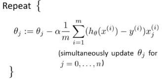
通过简单的求导后可得：

补充笔记

Gradient Descent for Multiple Variables

The gradient descent equation itself is generally the same form; we just have to repeat it for our 'n' features:

In other words:

The following image compares image compares gradient descent with one value to gradient descent with multiple variables:

特征缩放（Feature Scaling）

在多维特征的情况下，若我们保证这些特征都具有相近的尺度，则梯度下降算法能够更快地收敛。

我们还是以房价预测为例，假设此处我们只使用两个特征，房屋的面积和房间的数量，房屋面积的取值范围为0~2000平方英尺，房间数量的取值范围为0~5。同时，我们以两个参数为横、纵坐标轴构建代价函数的等高线图。

从图中可看出，椭圆较扁，且根据图中红色线条可知，梯度下降算法需要较多次数迭代才能收敛。

因此，为了让梯度下降算法更快的收敛，我们采用特征缩放和均值归一化的方法。特征缩放通过将特征变量除以特征变量的范围（即最大值减去最小值）的方法，使得特征变量的新取值范围仅为1，即-1 ≤ x_(i) ≤1；均值归一化通过特征变量的值减去特征变量的平均值的方法，使得特征变量的新平均值为0。我们通常使用如下公式实现特征缩放和均值归一化：

其中μ_n表示某一特征的平均值，s_n表示某一特征的标准差（或最大值与最小值间的差，即max-min）。

补充笔记

Feature Scaling

We can speed up gradient descent by having each of our input values in roughly the same range. This is because θ will descend quickly on small ranges and slowly on large ranges, and so will oscillate inefficiently down to the optimum when the variables are very uneven.

The way to prevent this is to modify the ranges of our input variables so that they are all roughly the same. Ideally:
　　-1 ≤ x_(i) ≤1
or
　　-0.5 ≤ x_(i) ≤0.5

These aren't exact requirements; we are only trying to speed things up. The goal is to get all input variables into roughly one of these ranges, give or take a few.

Two techniques to help with this are feature scaling and mean normalization. Feature scaling involves dividing the input values by the range (i.e. the maximum value minus the minimum values) of the input variable, resulting in a new range of just 1. Mean normalization involves subtracting the average value for an input variable from the values for that input variable resulting in a new average value for the input variable of just zero. To implement both of these techniques, adjust your input values as shown in this formula:

Where μ_i is the average of all the values for feature (i) and s_i is the range of values (max - min), or s_i is the standard deviation.

Note that dividing by the range, or dividing by the standard deviation, give different results.

学习率α

梯度下降算法收敛所需要的迭代次数根据模型的不同而不同。实际上，我们很难提前判断梯度下降算法需要多少步迭代才能收敛。对此，我们通常画出代价函数随着迭代步数增加的变化曲线来试着预测梯度下降算法是否已经收敛。

同时，这是种方法也可以进行一些自动收敛测试。（注：自动收敛测试就是用一种算法来判断梯度下降算法是否收敛，通常要选择一个合理的阈值ε来与代价函数J(θ)的下降的幅度比较，如若代价函数J(θ)的下降的幅度小于这个阈值ε，则可判断梯度下降算法已经收敛。但这个阈值ε的选择是非常困难的，因此我们实际上还是通过观察曲线图来判断梯度下降算法是否收敛。）

梯度下降算法的每次迭代都要受到学习率α的影响，当学习率α过小时，则梯度下降算法要进行很多次迭代才能收敛；当学习率α过大时，则梯度下降算法可能就会出错，即每次迭代，代价函数可能不会下降，并可能越过局部最小值导致无法收敛。

补充笔记

Learning Rate

Debugging gradient descent. Make a plot with number of iterations on the x-axis. Now plot the cost function, J(θ) over the number of iterations of gradient descent. If J(θ) ever increase, then you probably need to decrease α.

Automatic convergence test. Declare convergence if J(θ) decrease by less than E in one iteration, where E is some small value such as 10^-3. However in practice it's difficult to choose this threshold value.

It has been proven that if learning rate α is sufficiently small, then J(θ) will decrease on every iteration.

To summarize:

• if α is too small: slow convergence.
• if α is too large: may not decrease on every iteration and thus may not converge.

特征和多项式回归（Features and Polynomial Regression）

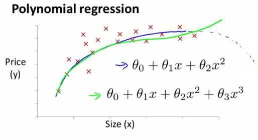
之前我们介绍了多变量的线性回归，现在我们来学习一下多项式回归，其能帮助我们使用线性回归的方法来拟合非常复杂的函数，甚至是非线性函数。

比如有时我们想使用二次方模型（h_θ(x) = θ₀ + θ₁x₁ + θ₂x₂²）来拟合我们的数据，又有时我们想使用三次方模型（h_θ(x) = θ₀ + θ₁x₁ + θ₂x₂² + θ₃x₃³）来拟合我们的数据······

通常我们需要先观察数据然后来决定参数使用什么样的模型。

另外，我们可以令：

• x₂ = x₂²
• x₃ = x₃³
  ······

这样我们就将这些多项式回归模型又转换为线性回归模型。（注：我们在使用多项式回归模型时，由于会对变量x_i进行平方、立方等操作，因此我们有必要在运行梯度下降算法之前进行特征缩放。）

补充笔记

Features and Polynomial Regression

We can improve our features and the form of our hypothesis function in a couple different ways.

We can combine multiple features into one. For example, we can combine x₁ and x₂ into a new feature x₃ by taking x₁ * x₂.

Polynomial Regression

Our hypothesis function need not be linear (a straight line) if that does not fit the data well.

We can change the behavior or curve of our hypothesis function by making it a quadratic, cubic or square root function (or any other form).

For example, if our hypothesis function is h_θ(x) = θ₀ + θ₁x₁ then we can create additional features based on x₁, to get the quadratic function h_θ(x) = θ₀ + θ₁x₁ + θ₂x₁² or the cubic function h_θ(x) = θ₀ + θ₁x₁ + θ₂x₁² + θ₃x₁³

In the cubic version, we have created new features x₂ = x₁² and x₃ = x₁³.

To make it a square root function, we could do:

One important thing to keep in mind is, if you choose your features this way then feature scaling becomes very important.

eg. if x₁ has range 1~1000 then range of x₁² becomes 1~1000000 and that of x₁³ becomes 1~1000000000