Factorization Machines

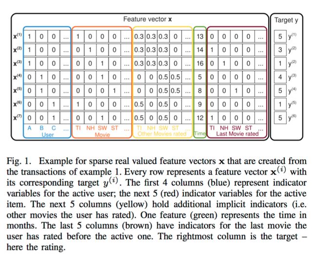
Feature Vector in Section 2
dependent interaction factor matrix in Section 3
complexity from in Section 3.A.4

1. INTRODUCTION

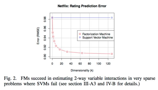
Standard SVM predictors are not successful in these tasks is that they cannot learn reliable parameters ('hyperplanes') in complex (non-linear) kernel spaces under very sparse data
the drawback of tensor factorization models and even more for specialized factorization models is that (1) they are not applicable to standard prediction data (e.g. a real valued feature vector in ) and (2) that specialized models are usually derived individually for a specific task requiring effort in modelling and design of a learning algorithm

the advantages of our proposed FM are:

FMs allow parameter estimation under very sparse data where SVMs fail
FMs have linear complexity, can be optimized in the primal and do not rely on support vectors like SVMs
FMs are a general predictor that can work with any real valued feature vector

2. PREDICTION UNDER SPARSITY

Let be the number of non-zero elements in the feature vector and be the average number of non-zero elements of all vectors . Huge sparsity () appears in many real-world data like feature vectors of event transactions

FM_feature.png

3. FACTORIZATION MACHINES

A. Factorization Machine Model

1. Model Equation

The model equation for a factorizationmachine of degree is defined as:

where the model parameters that have to be estimated are:

And is the dot product of two vectors of size :

A row within describes the -th variable with factors. is a hyperparameter that defines the dimensionality of the factorization

A 2-way FM (degree ) captures all single and pairwise interactions between variables:

is the global bias
models the strength of the -th variable
models the interaction between the -th and -th variable. Instead of using an own model parameter for each interaction, the FM models the interaction by factorizing it. We will see later on, that this is the key point which allows high quality parameter estimates of higher-order interactions () under sparsity

2. Expressiveness

It is well known that for any positive definite matrix , there exists a matrix such that provided that is sufficiently large. This shows that a FM can express any interaction matrix if is chosen large enough. Nevertheless in sparse settings, typically a small should be chosen because there is not enough data to estimate complex interactions . Restricting – and thus the expressiveness of the FM – leads to better generalization and thus improved interaction matrices under sparsity

3. Parameter Estimation Under Sparsity

Q: In sparse settings, there is usually not enough data to estimate interactions between variables directly and independently ?

A: Factorization machines can estimate interactions even in these settings well because they break the independence of the interaction parameters by factorizing them

one interaction helps also to estimate the parameters for related interactions

eg: Assume we want to estimate the interaction between Alice (A) and Star Trek (ST) for predicting the target (here the rating)

there is no case in the training data where both variables and are non-zero and thus a direct estimate would lead to no interaction ()
But with the factorized interaction parameters we can estimate the interaction even in
this case

reason:

First of all, Bob and Charlie will have similar factor vectors and because both have similar interactions with Star Wars () for predicting ratings – i.e. and have to be similar. Alice () will have a different factor vector from Charlie () because she has different interactions with the factors of Titanic and Star Wars for predicting ratings
Next, the factor vectors of Star Trek are likely to be similar to the one of Star Wars because Bob has similar interactions for both movies for predicting . In total, this means that the dot product (i.e. the interaction) of the factor vectors of Alice and Star Trek will be similar to the one of Alice and Star Wars – which also makes intuitively sense

4. Computation

Lemma 3.1: The model equation of a factorization machine (eq. (1)) can be computed in linear time

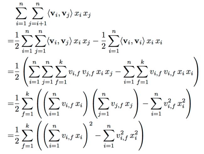
Proof: Due to the factorization of the pairwise interactions, there is no model parameter that directly depends on two variables (e.g. a parameter with an index ). So the pairwise interactions can be reformulated: ()

fm_computation.png

Moreover, under sparsity most of the elements in are (i.e. is small) and thus, the sums have only to be computed over the non-zero elements. Thus in sparse applications, the computation of the factorization machine is in – e.g. for typical recommender systems like MF approaches (see section 5-A)

B. Factorization Machines as Predictors

FM can be applied to a variety of prediction tasks. Among them are:

Regression: can be used directly as the predictor and the optimization criterion is e.g. the minimal least square error on
Binary classification: the sign of is used and the parameters are optimized for hinge loss or logit loss
Ranking: the vectors are ordered by the score of and optimization is done over pairs of instance vectors with a pairwise classification loss

In all these cases, regularization terms like are usually added to the optimization objective to prevent overfitting

C. Learning Factorization Machines

The gradient of the FM model is:
$\frac{\partial}{\partial\theta}\hat{y}(\mathbf{x})= \begin{cases} 1 & \text{if }\;\theta\;\text{ is }w_0 \\ x_i & \text{if } \;\theta\;\text{ is }w_i \\ x_i\sum^n_{j=1}v_{j,f}x_j-v_{i,f}x_i^2 & \text{if }\;\theta\;\text{ is } v_{i,j} \end{cases} \tag{4}$
The sum is independent of and thus can be precomputed (e.g. when computing ). In general, each gradient can be computed in constant time . And all parameter updates for a case can be done in – or under sparsity.

D. d-way Factorization Machine

The 2-way FM described so far can easily be generalized to a d-way FM:

where the interaction parameters for the -th interaction are factorized by the PARAFAC model [1] with the model parameters:

The straight-forward complexity for computing eq. (5) is . But with the same arguments as in lemma 3.1, one can show that it can be computed in linear time

E. Summary

FMs model all possible interactions between values in the feature vector using factorized interactions instead of full parametrized ones. This has two main advantages:

The interactions between values can be estimated even under high sparsity. Especially, it is possible to generalize to unobserved interactions
The number of parameters as well as the time for prediction and learning is linear. This makes direct optimization using SGD feasible and allows optimizing against a variety of loss functions

4. FMS VS. SVMS

1. SVM model

where is a mapping from the feature space into a more complex space . The mapping is related to a kernel with:

In the following, we discuss the relationships of FMs and SVMs by analyzing the primal form of the SVMs

kind	linear kernel	polynomial

		when

compared with FM	identical to a FM of degree	all interaction parameters of SVM are completely independent, the interaction parameters of FMs are factorized and thus and depend on each other as they overlap and share parameters

2. Parameter Estimation Under Sparsity

In the following, we will show why linear and polynomial SVMs fail for very sparse problems. We show this for the example of collaborative filtering with user and item indicator variables (see the first two groups (blue and red) in the example of figure 1). Here, the feature vectors are sparse and only two elements are non-zero (the active user and active item )

kind	linear kernel	polynominal

	This model corresponds to one of the most basic collaborative filtering models where only the user and item biases are captured. As this model is very simple, the parameters can be estimated well even under sparsity. However, the empirical prediction quality typically is low	estimating higher-order interactions is not only an issue in CF but in all scenarios where the data is hugely sparse. Because for a reliable estimate of the parameter of a pairwise interaction , there must be 'enough' cases where

facet	SVM	FM
sparsity	requires direct observations for the interactions	can be estimated well even under sparsity
solver	dual	primal
training data	depends on parts of the training data (the support vectors)	independent

fm_vs_svm.png

5. FMS VS. OTHER FACTORIZATION MODELS

There is a variety of factorization models, ranging from:

standard models for m-ary relations over categorical variables (e.g. MF, PARAFAC)
to specialized models for specific data and tasks (e.g. SVD++, PITF, FPMC)

Next, we show that FMs can mimic many of these models just by using the right input data (e.g. feature vector )

ref: https://www.csie.ntu.edu.tw/~b97053/paper/Rendle2010FM.pdf