局部加权回归（LOWESS）

局部加权线性回归：local weighted regression

核函数

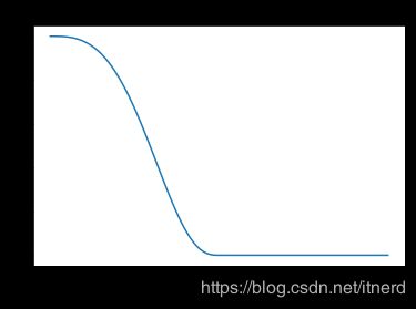
叶帕涅奇尼科夫（epanechnikov）核函数

又称二次核
$$K_l(x,x_0)=D(\frac{||x-x_0||}{l})$$
$$D(t)=\{\begin{array}{ll}0.75(1-t^2),& |t|<1,\\ 0,& otherwise.\end{array}$$

# Kernel functions:
def epanechnikov(xx, **kwargs):
    """
    The Epanechnikov kernel estimated for xx values at indices idx (zero
    elsewhere) 

    Parameters
    ----------
    xx: float array
        Values of the function on which the kernel is computed. Typically,
        these are Euclidean distances from some point x0 (see do_kernel)
    """
    l = kwargs.get('l', 1.0)
    ans = np.zeros(xx.shape)
    xx_norm = xx / l
    idx = np.where(xx_norm <= 1)
    ans[idx] = 0.75 * (1 - xx_norm[idx]  ** 2)
    return ans

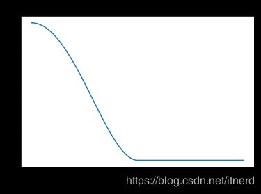
立方核

$$K_l(x,x_0)=D(\frac{||x-x_0||}{l})$$
$$D(t)=\{\begin{array}{ll}(1-|t{|}^3{)}^3,& |t|<1,\\ 0,& otherwise.\end{array}$$

def tri_cube(xx, **kwargs):
    """ 
    The tri-cube kernel estimated for xx values at indices idx (zero
    elsewhere) 

    Parameters
    ----------
    xx: float array
        Values of the function on which the kernel is computed. Typically,
        these are Euclidean distances from some point x0 (see do_kernel)

    idx: tuple
        An indexing tuple pointing to the coordinates in xx for which the
        kernel value is estimated. Default: None (all points are used!)       
    """
    ans = np.zeros(xx.shape)
    idx = np.where(xx <= 1)
    ans[idx] = (1 - np.abs(xx[idx]) ** 3) ** 3
    return ans

应用核函数

$$do\_kernel=kernel(||x-x_0|{|}_2;l)$$

def do_kernel(x0, x, l=1.0, kernel=epanechnikov):
    """
    Calculate a kernel function on x in the neighborhood of x0

    Parameters
    ----------
    x: float array
       All values of x
    x0: float
       The value of x around which we evaluate the kernel
    l: float or float array (with shape = x.shape)
       Width parameter (metric window size)
    kernel: callable
        A kernel function. Any function with signature: `func(xx)`    
    """
    # xx is the norm of x-x0. Note that we broadcast on the second axis for the
    # nd case and then sum on the first to get the norm in each value of x:
    xx = np.sum(np.sqrt(np.power(x - x0[:, np.newaxis], 2)), 0)
    return kernel(xx, l=l)

局部加权回归

拟合函数
$$f(x)=\sum _{i=0}^d{\alpha }_i{x}^i$$
优化目标
$$\underset{\alpha }{\min }\sum _{i=1}^{N}K(x,x_i){\left(y_i-\sum _{j=0}^d{\alpha }_j{x}^j\right)}^2$$
写成矩阵形式
$$\underset{A}{\min }(Y-XA{)}^{\top }K(Y-XA)$$
解得：
$$A=(X^{\top }KX{)}^{-1}{X}^{\top }KY$$

增强鲁棒性

双平方函数

用双平方函数来降低异常点的影响，见下一节。

双平方函数为
$$B(t)=\{\begin{array}{ll}(1-t^2{)}^2,& |t|<1,\\ 0,& otherwise.\end{array}$$

def bi_square(xx, **kwargs):
    """
    The bi-square weight function calculated over values of xx

    Parameters
    ----------
    xx: float array
    """
    ans = np.zeros(xx.shape)
    idx = np.where(xx < 1)
    ans[idx] = (1 - xx[idx] ** 2) ** 2
    return ans

鲁棒局部加权线性回归

先做一次局部加权回归，计算出拟合的残差：
$$e_i=y_i-f(x_i)$$
利用双平方函数计算误差权重：
$${\delta }_i=B(e_i/6s)$$
其中 $s$ 为误差绝对值 $|e_i|$ 的中位数，上式的含义是将误差大于6倍中位数的点视为离群点，权重赋为 0.

将 ${\delta }_i$ 乘以核函数得到的距离权重 $K(x,x_i)$，再做一次加权回归。

def lowess(x, y, x0, deg=1, kernel=epanechnikov, l=1, robust=False,):
    """
    Locally smoothed regression with the LOWESS algorithm.

    Parameters
    ----------
    x: float n-d array  
       Values of x for which f(x) is known (e.g. measured). The shape of this
       is (n, j), where n is the number the dimensions and j is the
       number of distinct coordinates sampled.
    
    y: float array
       The known values of f(x) at these points. This has shape (j,) 

    x0: float or float array.
        Values of x for which we estimate the value of f(x). This is either a
        single scalar value (only possible for the 1d case, in which case f(x0)
        is estimated for just that one value of x), or an array of shape (n, k).

    deg: int
        The degree of smoothing functions. 0 is locally constant, 1 is locally
        linear, etc. Default: 1.
        
    kernel: callable
        A kernel function. {'epanechnikov', 'tri_cube', 'bi_square'}

    l: float or float array with shape = x.shape
       The metric window size for the kernel

    robust: bool
        Whether to apply the robustification procedure from [Cleveland79], page
        831
    
        
    Returns
    -------
    The function estimated at x0. 
    """
    if robust:
        # We use the procedure described in Cleveland1979
        # Start by calling this function with robust set to false and the x0
        # input being equal to the x input:
        y_est = lowess(x, y, x, kernel=epanechnikov, l=l, robust=False)
        resid = y_est - y
        median_resid = np.nanmedian(np.abs(resid))
        # Calculate the bi-cube function on the residuals for robustness
        # weights: 
        robustness_weights = bi_square(resid / (6 * median_resid))
        
    # For the case where x0 is provided as a scalar: 
    if not np.iterable(x0):
       x0 = np.asarray([x0])
    ans = np.zeros(x0.shape[-1]) 
    # We only need one design matrix for fitting:
    B = [np.ones(x.shape[-1])]
    for d in range(1, deg+1):
        B.append(x ** deg)

    B = np.vstack(B).T
    for idx, this_x0 in enumerate(x0.T):
        # This is necessary in the 1d case (?):
        if not np.iterable(this_x0):
            this_x0 = np.asarray([this_x0])
        # Different weighting kernel for each x0:
        W = np.diag(do_kernel(this_x0, x, l=l, kernel=kernel))
        # XXX It should be possible to calculate W outside the loop, if x0 and
        # x are both sampled in some regular fashion (that is, if W is the same
        # matrix in each iteration). That should save time.

        if robust:
            # We apply the robustness weights to the weighted least-squares
            # procedure:
            robustness_weights[np.isnan(robustness_weights)] = 0
            W = np.dot(W, np.diag(robustness_weights))

        BtWB = np.dot(np.dot(B.T, W), B)
        BtW = np.dot(B.T, W)
        # Get the params:
        beta = np.dot(np.dot(la.pinv(BtWB), BtW), y.T)
        # We create a design matrix for this coordinat for back-predicting:
        B0 = [1]
        for d in range(1, deg+1):
            B0 = np.hstack([B0, this_x0 ** deg])
        B0 = np.vstack(B0).T
        # Estimate the answer based on the parameters:
        ans[idx] += np.dot(B0, beta)
    # If we are trying to sample far away from where the function is
    # defined, we will be trying to invert a singular matrix. In that case,
    # the regression should not work for you and you should get a nan:
        #except la.LinAlgError :
        #    ans[idx] += np.nan
    return ans.T