TensorFlow 实现多层 LSTM 的 MNIST 分类 + 可视化

前言

循环神经网络（recurrent neural networks, RNNs）及其改进算法长短期记忆网络（Long Short-Term Memory, LSTM）能够很好地对时序数据进行建模，其的相关基础不进行介绍，需要了解可以参考以下文章：
Understanding LSTM Networks
RNN快速入门
YJango的循环神经网络——实现LSTM
莫烦 PYTHON：什么是循环神经网络 RNN

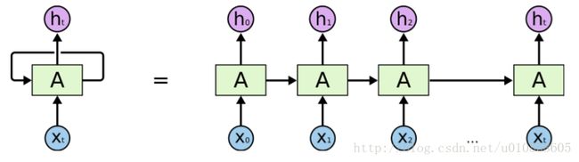
RNNs 展开示意图：

LSTM 结构示意图：

TensorFlow 实现

采用两层的 LSTM 实现对 MNIST 手写数字进行分类，并对训练过程中的误差和准确率进行 tensorboard 的可视化。

1. 初始化参数

这里 mnist 图像尺寸是 28*28 的，可以看作时序长度 28（图像的宽），输入为 28（图像的高）

# Hyper Parameters
learning_rate = 0.01    # 学习率
n_steps = 28            # LSTM 展开步数（时序持续长度）
n_inputs = 28           # 输入节点数
n_hiddens = 64         # 隐层节点数
n_layers = 2            # LSTM layer 层数
n_classes = 10          # 输出节点数（分类数目）

2. 定义输入输出的 placeholder

# tensor placeholder
with tf.name_scope('inputs'):
    x = tf.placeholder(tf.float32, [None, n_steps * n_inputs], name='x_input')     # 输入
    y = tf.placeholder(tf.float32, [None, n_classes], name='y_input')               # 输出
    keep_prob = tf.placeholder(tf.float32, name='keep_prob_input')           # 保持多少不被 dropout
    batch_size = tf.placeholder(tf.int32, [], name='batch_size_input')       # 批大小

3. 定义网络的权重和偏置

# weights and biases
with tf.name_scope('weights'):
    Weights = tf.Variable(tf.truncated_normal([n_hiddens, n_classes],stddev=0.1), dtype=tf.float32, name='W')
    tf.summary.histogram('output_layer_weights', Weights)
with tf.name_scope('biases'):
    biases = tf.Variable(tf.random_normal([n_classes]), name='b')
    tf.summary.histogram('output_layer_biases', biases)

4. RNN 网络结构

# RNN structure
def RNN_LSTM(x, Weights, biases):
    # RNN 输入 reshape
    x = tf.reshape(x, [-1, n_steps, n_inputs])
    # 定义 LSTM cell
    # cell 中的 dropout
    def attn_cell():
        lstm_cell = tf.contrib.rnn.BasicLSTMCell(n_hiddens)
        with tf.name_scope('lstm_dropout'):
            return tf.contrib.rnn.DropoutWrapper(lstm_cell, output_keep_prob=keep_prob)
    # attn_cell = tf.contrib.rnn.DropoutWrapper(lstm_cell, output_keep_prob=keep_prob)
    # 实现多层 LSTM
    # [attn_cell() for _ in range(n_layers)]
    enc_cells = []
    for i in range(0, n_layers):
        enc_cells.append(attn_cell())
    with tf.name_scope('lstm_cells_layers'):
        mlstm_cell = tf.contrib.rnn.MultiRNNCell(enc_cells, state_is_tuple=True)
    # 全零初始化 state
    _init_state = mlstm_cell.zero_state(batch_size, dtype=tf.float32)
    # dynamic_rnn 运行网络
    outputs, states = tf.nn.dynamic_rnn(mlstm_cell, x, initial_state=_init_state, dtype=tf.float32, time_major=False)
    # 输出
    #return tf.matmul(outputs[:,-1,:], Weights) + biases
    return tf.nn.softmax(tf.matmul(outputs[:,-1,:], Weights) + biases)

5. 损失函数和优化器

with tf.name_scope('output_layer'):
    pred = RNN_LSTM(x, Weights, biases)
    tf.summary.histogram('outputs', pred)
# cost
with tf.name_scope('loss'):
    #cost = tf.reduce_mean(tf.nn.softmax_cross_entropy_with_logits(logits=pred, labels=y))
    cost = tf.reduce_mean(-tf.reduce_sum(y * tf.log(pred),reduction_indices=[1]))
    tf.summary.scalar('loss', cost)
# optimizer
with tf.name_scope('train'):
    train_op = tf.train.AdamOptimizer(learning_rate=learning_rate).minimize(cost)

# correct_pred = tf.equal(tf.argmax(pred, 1), tf.argmax(y, 1))
# accuarcy = tf.reduce_mean(tf.cast(correct_pred, tf.float32))
with tf.name_scope('accuracy'):
    accuracy = tf.metrics.accuracy(labels=tf.argmax(y, axis=1), predictions=tf.argmax(pred, axis=1))[1]
    tf.summary.scalar('accuracy', accuracy)

merged = tf.summary.merge_all()

init = tf.group(tf.global_variables_initializer(), tf.local_variables_initializer())

6. 训练

with tf.Session() as sess:
    sess.run(init)
    train_writer = tf.summary.FileWriter("E://logs//train",sess.graph)
    test_writer = tf.summary.FileWriter("E://logs//test",sess.graph)
    # training
    step = 1
    for i in range(2000):
        _batch_size = 128
        batch_x, batch_y = mnist.train.next_batch(_batch_size)

        sess.run(train_op, feed_dict={x:batch_x, y:batch_y, keep_prob:0.5, batch_size:_batch_size})
        if (i + 1) % 100 == 0:
            train_result = sess.run(merged, feed_dict={x:batch_x, y:batch_y, keep_prob:1.0, batch_size:_batch_size})
            test_result = sess.run(merged, feed_dict={x:test_x, y:test_y, keep_prob:1.0, batch_size:test_x.shape[0]})
            train_writer.add_summary(train_result,i+1)
            test_writer.add_summary(test_result,i+1)

    print("Optimization Finished!")

7. 预测

    test_x = mnist.test.images
    test_y = mnist.test.labels
    # prediction
    print("Testing Accuracy:", sess.run(accuracy, feed_dict={x:test_x, y:test_y, keep_prob:1.0, batch_size:test_x.shape[0]}))

可视化结果

训练集和测试集的在训练过程中的误差变化对比：

训练集和测试集的在训练过程中的预测准确率对比：

附全部代码

import tensorflow as tf
from tensorflow.examples.tutorials.mnist import input_data

tf.reset_default_graph()

# Hyper Parameters
learning_rate = 0.01    # 学习率
n_steps = 28            # LSTM 展开步数（时序持续长度）
n_inputs = 28           # 输入节点数
n_hiddens = 64         # 隐层节点数
n_layers = 2            # LSTM layer 层数
n_classes = 10          # 输出节点数（分类数目）

# data
mnist = input_data.read_data_sets("E:/Anaconda3/workspace/MNIST_data/", one_hot=True)
test_x = mnist.test.images
test_y = mnist.test.labels

# tensor placeholder
with tf.name_scope('inputs'):
    x = tf.placeholder(tf.float32, [None, n_steps * n_inputs], name='x_input')     # 输入
    y = tf.placeholder(tf.float32, [None, n_classes], name='y_input')               # 输出
    keep_prob = tf.placeholder(tf.float32, name='keep_prob_input')           # 保持多少不被 dropout
    batch_size = tf.placeholder(tf.int32, [], name='batch_size_input')       # 批大小

# weights and biases
with tf.name_scope('weights'):
    Weights = tf.Variable(tf.truncated_normal([n_hiddens, n_classes],stddev=0.1), dtype=tf.float32, name='W')
    tf.summary.histogram('output_layer_weights', Weights)
with tf.name_scope('biases'):
    biases = tf.Variable(tf.random_normal([n_classes]), name='b')
    tf.summary.histogram('output_layer_biases', biases)

# RNN structure
def RNN_LSTM(x, Weights, biases):
    # RNN 输入 reshape
    x = tf.reshape(x, [-1, n_steps, n_inputs])
    # 定义 LSTM cell
    # cell 中的 dropout
    def attn_cell():
        lstm_cell = tf.contrib.rnn.BasicLSTMCell(n_hiddens)
        with tf.name_scope('lstm_dropout'):
            return tf.contrib.rnn.DropoutWrapper(lstm_cell, output_keep_prob=keep_prob)
    # attn_cell = tf.contrib.rnn.DropoutWrapper(lstm_cell, output_keep_prob=keep_prob)
    # 实现多层 LSTM
    # [attn_cell() for _ in range(n_layers)]
    enc_cells = []
    for i in range(0, n_layers):
        enc_cells.append(attn_cell())
    with tf.name_scope('lstm_cells_layers'):
        mlstm_cell = tf.contrib.rnn.MultiRNNCell(enc_cells, state_is_tuple=True)
    # 全零初始化 state
    _init_state = mlstm_cell.zero_state(batch_size, dtype=tf.float32)
    # dynamic_rnn 运行网络
    outputs, states = tf.nn.dynamic_rnn(mlstm_cell, x, initial_state=_init_state, dtype=tf.float32, time_major=False)
    # 输出
    #return tf.matmul(outputs[:,-1,:], Weights) + biases
    return tf.nn.softmax(tf.matmul(outputs[:,-1,:], Weights) + biases)

with tf.name_scope('output_layer'):
    pred = RNN_LSTM(x, Weights, biases)
    tf.summary.histogram('outputs', pred)
# cost
with tf.name_scope('loss'):
    #cost = tf.reduce_mean(tf.nn.softmax_cross_entropy_with_logits(logits=pred, labels=y))
    cost = tf.reduce_mean(-tf.reduce_sum(y * tf.log(pred),reduction_indices=[1]))
    tf.summary.scalar('loss', cost)
# optimizer
with tf.name_scope('train'):
    train_op = tf.train.AdamOptimizer(learning_rate=learning_rate).minimize(cost)

# correct_pred = tf.equal(tf.argmax(pred, 1), tf.argmax(y, 1))
# accuarcy = tf.reduce_mean(tf.cast(correct_pred, tf.float32))
with tf.name_scope('accuracy'):
    accuracy = tf.metrics.accuracy(labels=tf.argmax(y, axis=1), predictions=tf.argmax(pred, axis=1))[1]
    tf.summary.scalar('accuracy', accuracy)

merged = tf.summary.merge_all()

init = tf.group(tf.global_variables_initializer(), tf.local_variables_initializer())

with tf.Session() as sess:
    sess.run(init)
    train_writer = tf.summary.FileWriter("E://logs//train",sess.graph)
    test_writer = tf.summary.FileWriter("E://logs//test",sess.graph)
    # training
    step = 1
    for i in range(2000):
        _batch_size = 128
        batch_x, batch_y = mnist.train.next_batch(_batch_size)

        sess.run(train_op, feed_dict={x:batch_x, y:batch_y, keep_prob:0.5, batch_size:_batch_size})
        if (i + 1) % 100 == 0:
            #loss = sess.run(cost, feed_dict={x:batch_x, y:batch_y, keep_prob:1.0, batch_size:_batch_size})
            #acc = sess.run(accuracy, feed_dict={x:batch_x, y:batch_y, keep_prob:1.0, batch_size:_batch_size})
            #print('Iter: %d' % ((i+1) * _batch_size), '| train loss: %.6f' % loss, '| train accuracy: %.6f' % acc)
            train_result = sess.run(merged, feed_dict={x:batch_x, y:batch_y, keep_prob:1.0, batch_size:_batch_size})
            test_result = sess.run(merged, feed_dict={x:test_x, y:test_y, keep_prob:1.0, batch_size:test_x.shape[0]})
            train_writer.add_summary(train_result,i+1)
            test_writer.add_summary(test_result,i+1)

    print("Optimization Finished!")
    # prediction
    print("Testing Accuracy:", sess.run(accuracy, feed_dict={x:test_x, y:test_y, keep_prob:1.0, batch_size:test_x.shape[0]}))