geopandas地图数据可视化

geopandas安装

Anaconda3集成环境下，直接在anaconda prompt 命令窗口执行 conda install -c conda-forge geopandas
就会自动进行下载安装。

可视化流程

1. 数据准备

.geojson类型的文件一个是必须的，本文使用的数据有neighbourhoods.geojson，listings.csv。前者为北京16个区域的形状信息，后者为各区域的短租房信息。

本文使用数据链接

2. 导入数据

import pandas as pd
import numpy as np
import pandas as pd
import matplotlib.pyplot as plt
import geopandas as gpd
from shapely.geometry import Point # 经纬度转换为点
import adjustText as aT
import mapclassify
%pylab inline
%matplotlib inline
plt.rcParams['font.sans-serif'] = ['SimHei']
plt.rcParams['axes.unicode_minus'] = False
import warnings
warnings.filterwarnings('ignore')

导入形状

geo_ = gpd.GeoDataFrame.from_file('E:/tianchi/neighbourhoods.geojson') #读取数据为geodataframe格式
geo_=geo_.drop("neighbourhood_group",axis=1)#清洗
geo['neighbourhood'] = geo['neighbourhood'].apply(lambda x: x.split('/')[0].strip())#统一中文名称
geo_.head(3)

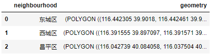
neighbourhood这一列代表北京的16个地区的名字，geometry这一列存放着各区的形状。

导入各地区房屋的信息

df=pd.read_csv('E:/tianchi/listings.csv')#有这一句就够了，后面的是一些数据清洗，我这里保留了

df=df[df['availability_365']>0]
df=df.drop("neighbourhood_group",axis=1)
df=df[df["minimum_nights"]<=365]
df['neighbourhood'] = df['neighbourhood'].apply(lambda x: x.split('/')[0].strip())
for i in df['neighbourhood'].unique():
    for j in df['room_type'].unique():
        Q75=df[df['neighbourhood']==i][df['room_type']==j]['price'].quantile(0.75)
        Q25=df[df['neighbourhood']==i][df['room_type']==j]['price'].quantile(0.25)
        iqr=Q75-Q25
        df.loc[(df['neighbourhood']==i) & (df['room_type']==j),'上限']=Q75+1.5*iqr
        df.loc[(df['neighbourhood']==i) & (df['room_type']==j),'下限']=Q25-1.5*iqr
df=df[(df['price']>=df['下限'])&(df['price']<=df['上限'])]
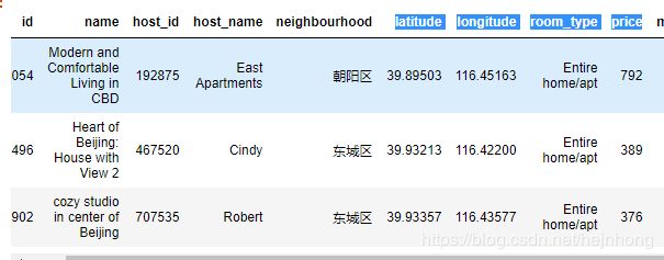
df.head(3)

latitude、longitude、price是我们需要用的有用信息，通过经纬度，我们能在地图上描出房屋的分布。

3. 绘制图形

geo_.plot()

           这就是北京市的形状以及区域划分

（1）把经纬度转化为坐标

df['geometry']=list(zip(df['longitude'],df['latitude']))#经纬度组合为新列geometry，与形状里的该列对应
df['geometry']=df['geometry'].apply(Point)#经纬度转化为坐标点
gpd_df=gpd.GeoDataFrame(df)

新增了一列geometry，与geo_里的geometry对应，画图时自动关联

（2）在底图上描点

base = geo_.plot(color='lightblue', edgecolor='grey',figsize=(15, 15))#利用形状信息画底图
gpd_df.plot(ax=base, color='red', marker="o", markersize=50, alpha=0.01) #在底图上添加出租房位置
plt.gca().xaxis.set_major_locator(plt.NullLocator())#去掉x轴刻度
plt.gca().yaxis.set_major_locator(plt.NullLocator())#去掉y轴刻度

现在通过红点的疏密，我们已经能知道出租房的分布了

（3）地图颜色

地图颜色能表达很多信息，可以用来表示该区域的房屋数量或房屋价钱等信息，鉴于已经用红点表示房屋的分布了，这里就用颜色来代表各区域的出租房均价。

求均价

geo_price=df.groupby('neighbourhood')[['price']].mean()
geo_price.columns = ["mean"]

合并列

geo_merge = pd.merge(geo_, geo_price,on="neighbourhood", how="left")
geo_merge.head(5)

设置每块区域的代表点，以便添加label

geo_points=geo_merge.copy()
geo_points['center']=geo_points['geometry'].centroid#选取区域的中心点，添加列center
#nbhd_points['center']=nbhd_points['geometry'].representative_point()#另一种选取方法，不一定是中心点了
geo_points.set_geometry("center", inplace=True)

终于要绘图了

base = geo_merge.plot(column="mean", cmap='GnBu', scheme="boxplot",  #底图，颜色代表价格
                      edgecolor='grey',legend=True, figsize=(15, 15))
gpd_df.plot(ax=base, color='red', marker="o", markersize=50, alpha=0.01) #在底图上叠加房源点数据
plt.title("北京市房源分布图",fontsize=30)

texts = []  #标注区域名称
for x, y, label in zip(geo_points.geometry.x, geo_points.geometry.y,geo_points["neighbourhood"]):
    texts.append(plt.text(x, y, label, fontsize=12))

aT.adjust_text(texts,force_points=0.3, force_text=0.8, expand_points=(1, 1), expand_text=(1, 1),
               arrowprops=dict(arrowstyle="-", color='grey', lw=0.5))

plt.gca().xaxis.set_major_locator(plt.NullLocator())#去掉x轴刻度
plt.gca().yaxis.set_major_locator(plt.NullLocator())#去掉y轴刻度

结果挺漂亮的吧，在图示能直接看出各区域的房屋数量分布，还能看到各区域出租房的均价