线性回归

线性回归模型与诊断

数据说明：本数据是一份汽车贷款数据

字段名	中文含义
id	id
Acc	是否开卡(1=已开通)
avg_exp	月均信用卡支出（元）
avg_exp_ln	月均信用卡支出的自然对数
gender	性别(男=1)
Age	年龄
Income	年收入（万元）
Ownrent	是否自有住房（有=1；无=0)
Selfempl	是否自谋职业(1=yes, 0=no)
dist_home_val	所住小区房屋均价(万元)
dist_avg_income	当地人均收入
high_avg	高出当地平均收入
edu_class	教育等级：小学及以下开通=0，中学=1，本科=2，研究生=3

%matplotlib inline

import matplotlib.pyplot as plt
import os
import numpy as np
import pandas as pd
import statsmodels.api as sm
from statsmodels.formula.api import ols

os.chdir('E:/data')
pd.set_option('display.max_columns', 8)

E:\Anaconda3\lib\site-packages\statsmodels\compat\pandas.py:56: FutureWarning: The pandas.core.datetools module is deprecated and will be removed in a future version. Please use the pandas.tseries module instead.
  from pandas.core import datetools

导入数据和数据清洗

raw = pd.read_csv('creditcard_exp.csv', skipinitialspace=True)
raw.head()

	id	Acc	avg_exp	avg_exp_ln	...	dist_avg_income	age2	high_avg	edu_class
0	19	1	1217.03	7.104169	...	15.932789	1600	0.102361	3
1	5	1	1251.50	7.132098	...	15.796316	1024	0.051184	2
2	95	0	NaN	NaN	...	7.490000	1296	0.910000	1
3	86	1	856.57	6.752936	...	11.275632	1681	0.197218	3
4	50	1	1321.83	7.186772	...	13.346474	784	0.062676	2

5 rows × 14 columns

exp = raw[raw['avg_exp'].notnull()].copy().iloc[:, 2:]\
.drop('age2',axis=1)

exp_new = raw[raw['avg_exp'].isnull()].copy().iloc[:, 2:]\
.drop('age2',axis=1)

exp.describe(include='all')

	avg_exp	avg_exp_ln	gender	Age	...	dist_home_val	dist_avg_income	high_avg	edu_class
count	70.000000	70.000000	70.000000	70.000000	...	70.000000	70.000000	70.000000	70.000000
mean	983.655429	6.787787	0.285714	31.157143	...	74.540857	8.005472	-0.580766	1.928571
std	446.294237	0.476035	0.455016	7.206349	...	36.949228	3.070744	0.432808	0.873464
min	163.180000	5.094854	0.000000	20.000000	...	13.130000	3.828842	-1.526850	0.000000
25%	697.155000	6.547003	0.000000	26.000000	...	49.302500	5.915553	-0.887981	1.000000
50%	884.150000	6.784627	0.000000	30.000000	...	65.660000	7.084184	-0.612068	2.000000
75%	1229.585000	7.114415	1.000000	36.000000	...	105.067500	9.123105	-0.302082	3.000000
max	2430.030000	7.795659	1.000000	55.000000	...	157.900000	18.427000	0.259337	3.000000

8 rows × 11 columns

相关性分析

散点图

exp.plot('Income', 'avg_exp', kind='scatter')
plt.show()

[外链图片转存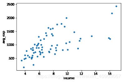(img-0SGvSTVL-1562725477539)(output_7_0.png)]

exp[['Income', 'avg_exp', 'Age', 'dist_home_val']].corr(method='pearson')

	Income	avg_exp	Age	dist_home_val
Income	1.000000	0.674011	0.369129	0.249153
avg_exp	0.674011	1.000000	0.258478	0.319499
Age	0.369129	0.258478	1.000000	0.109323
dist_home_val	0.249153	0.319499	0.109323	1.000000

线性回归算法

简单线性回归

lm_s = ols('avg_exp ~ Income', data=exp).fit()
print(lm_s.params)

Intercept    258.049498
Income        97.728578
dtype: float64

Predict-在原始数据集上得到预测值和残差

lm_s.summary()

OLS Regression Results

Dep. Variable:	avg_exp	R-squared:	0.454
Model:	OLS	Adj. R-squared:	0.446
Method:	Least Squares	F-statistic:	56.61
Date:	Mon, 30 Apr 2018	Prob (F-statistic):	1.60e-10
Time:	16:59:33	Log-Likelihood:	-504.69
No. Observations:	70	AIC:	1013.
Df Residuals:	68	BIC:	1018.
Df Model:	1
Covariance Type:	nonrobust

	coef	std err	t	P>|t|	[0.025	0.975]
Intercept	258.0495	104.290	2.474	0.016	49.942	466.157
Income	97.7286	12.989	7.524	0.000	71.809	123.648

Omnibus:	3.714	Durbin-Watson:	1.424
Prob(Omnibus):	0.156	Jarque-Bera (JB):	3.507
Skew:	0.485	Prob(JB):	0.173
Kurtosis:	2.490	Cond. No.	21.4

pd.DataFrame([lm_s.predict(exp), lm_s.resid], index=['predict', 'resid']
            ).T.head()

	predict	resid
0	1825.141904	-608.111904
1	1806.803136	-555.303136
3	1379.274813	-522.704813
4	1568.506658	-246.676658
5	1238.281793	-422.251793

在待预测数据集上得到预测值

lm_s.predict(exp_new)[:5]

2     1078.969552
11     756.465245
13     736.919530
19     687.077955
20     666.554953
dtype: float64

多元线性回归

lm_m = ols('avg_exp ~Income + dist_home_val + dist_avg_income',
           data=exp).fit()
lm_m.summary()

OLS Regression Results

Dep. Variable:	avg_exp	R-squared:	0.541
Model:	OLS	Adj. R-squared:	0.520
Method:	Least Squares	F-statistic:	25.95
Date:	Mon, 30 Apr 2018	Prob (F-statistic):	3.34e-11
Time:	16:59:33	Log-Likelihood:	-498.62
No. Observations:	70	AIC:	1005.
Df Residuals:	66	BIC:	1014.
Df Model:	3
Covariance Type:	nonrobust

	coef	std err	t	P>|t|	[0.025	0.975]
Intercept	2.3507	122.525	0.019	0.985	-242.278	246.980
Income	-164.4378	86.487	-1.901	0.062	-337.115	8.239
dist_home_val	1.5396	1.049	1.468	0.147	-0.555	3.634
dist_avg_income	260.7522	87.058	2.995	0.004	86.934	434.570

Omnibus:	5.379	Durbin-Watson:	1.593
Prob(Omnibus):	0.068	Jarque-Bera (JB):	5.367
Skew:	0.642	Prob(JB):	0.0683
Kurtosis:	2.563	Cond. No.	325.

exp.Income

0     16.03515
1     15.84750
3     11.47285
4     13.40915
5     10.03015
6     11.70575
7     11.81885
8      9.31260
9     16.28885
10     8.21290
12    10.31100
14    16.90015
15     9.81175
16     8.37990
17     9.57100
18     7.91000
22     8.36860
23     7.43320
25     6.62415
26     8.53830
27     6.67270
29    10.96410
30     7.37330
32     7.02025
34     9.13150
35     7.62235
39     6.14075
40     5.92290
41     7.93215
42     7.79915
        ...   
56     5.91685
57     5.04755
58     3.99125
60     4.91825
61     5.66840
62     5.80935
64     5.02000
67     7.78860
68     7.30525
69     6.07935
71     4.93595
72     4.90190
73     5.15780
74     6.35895
75     5.09540
76     5.89170
78     4.81890
80     5.06555
81     4.19345
82     4.62600
83     6.42760
84     6.17745
85     5.33175
87     5.44810
89     5.22925
93     4.05520
94     3.89305
96     4.37960
97     3.49390
98     3.81590
Name: Income, Length: 70, dtype: float64

多元线性回归的变量筛选

'''forward select'''
def forward_select(data, response):
    remaining = set(data.columns)
    remaining.remove(response)
    selected = []
    current_score, best_new_score = float('inf'), float('inf')
    while remaining:
        aic_with_candidates=[]
        for candidate in remaining:
            formula = "{} ~ {}".format(
                response,' + '.join(selected + [candidate]))
            aic = ols(formula=formula, data=data).fit().aic
            aic_with_candidates.append((aic, candidate))
        aic_with_candidates.sort(reverse=True)
        best_new_score, best_candidate=aic_with_candidates.pop()
        if current_score > best_new_score: 
            remaining.remove(best_candidate)
            selected.append(best_candidate)
            current_score = best_new_score
            print ('aic is {},continuing!'.format(current_score))
        else:        
            print ('forward selection over!')
            break
            
    formula = "{} ~ {} ".format(response,' + '.join(selected))
    print('final formula is {}'.format(formula))
    model = ols(formula=formula, data=data).fit()
    return(model)

data_for_select = exp[['avg_exp', 'Income', 'Age', 'dist_home_val', 
                       'dist_avg_income']]
lm_m = forward_select(data=data_for_select, response='avg_exp')
print(lm_m.rsquared)

aic is 1007.6801413968115,continuing!
aic is 1005.4969816306302,continuing!
aic is 1005.2487355956046,continuing!
forward selection over!
final formula is avg_exp ~ dist_avg_income + Income + dist_home_val 
0.541151292841195

线性回归的诊断

残差分析

ana1 = lm_s

exp['Pred'] = ana1.predict(exp)
exp['resid'] = ana1.resid
exp.plot('Income', 'resid',kind='scatter')
plt.show()

[外链图片转存(img-2JPBqa8G-1562725477554)(output_24_0.png)]

遇到异方差情况,教科书上会介绍使用加权最小二乘法，但是实际上最常用的是对被解释变量取对数

ana2 = ols('avg_exp_ln ~ Income', exp).fit()
exp['Pred'] = ana2.predict(exp)
exp['resid'] = ana2.resid
exp.plot('Income', 'resid',kind='scatter')
plt.show()

[外链图片转存(img-py8qc9gM-1562725477555)(output_26_0.png)]

取对数会使模型更有解释意义

exp['Income_ln'] = np.log(exp['Income'])

ana3 = ols('avg_exp_ln ~ Income_ln', exp).fit()
exp['Pred'] = ana3.predict(exp)
exp['resid'] = ana3.resid
exp.plot('Income_ln', 'resid',kind='scatter')
plt.show()

[外链图片转存(img-ETbm7yUC-1562725477555)(output_29_0.png)]

寻找最优的模型

r_sq = {'exp~Income':ana1.rsquared, 'ln(exp)~Income':ana2.rsquared, 
        'ln(exp)~ln(Income)':ana3.rsquared}
print(r_sq)

{'ln(exp)~Income': 0.4030855555329649, 'ln(exp)~ln(Income)': 0.4803927993893108, 'exp~Income': 0.45429062315565294}

强影响点分析

exp['resid_t'] = \
(exp['resid'] - exp['resid'].mean()) / exp['resid'].std()

Find outlier：

exp[abs(exp['resid_t']) > 2]

	avg_exp	avg_exp_ln	gender	Age	...	Pred	resid	Income_ln	resid_t
73	251.56	5.527682	0	29	...	6.526331	-0.998649	1.640510	-2.910292
98	163.18	5.094854	0	22	...	6.257191	-1.162337	1.339177	-3.387317

2 rows × 15 columns

Drop outlier

exp2 = exp[abs(exp['resid_t']) <= 2].copy()
ana4 = ols('avg_exp_ln ~ Income_ln', exp2).fit()
exp2['Pred'] = ana4.predict(exp2)
exp2['resid'] = ana4.resid
exp2.plot('Income', 'resid', kind='scatter')
plt.show()

[外链图片转存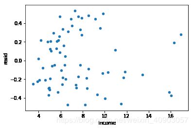(img-YVNFKJRc-1562725477556)(output_37_0.png)]

ana4.rsquared

0.49397191385172456

statemodels包提供了更多强影响点判断指标

from statsmodels.stats.outliers_influence import OLSInfluence

OLSInfluence(ana3).summary_frame().head()

	dfb_Intercept	dfb_Income_ln	cooks_d	dffits	dffits_internal	hat_diag	standard_resid	student_resid
0	0.343729	-0.381393	0.085587	-0.416040	-0.413732	0.089498	-1.319633	-1.326996
1	0.307196	-0.341294	0.069157	-0.373146	-0.371907	0.087409	-1.201699	-1.205702
3	0.207619	-0.244956	0.044984	-0.302382	-0.299947	0.041557	-1.440468	-1.452165
4	0.112301	-0.127713	0.010759	-0.145967	-0.146693	0.060926	-0.575913	-0.573062
5	0.120572	-0.150924	0.022274	-0.211842	-0.211064	0.029011	-1.221080	-1.225579

增加变量

经过单变量线性回归的处理，我们基本对模型的性质有了一定的了解，接下来可以放入更多的连续型解释变量。在加入变量之前，要注意变量的函数形式转变。比如当地房屋均价、当地平均收入，其性质和个人收入一样，都需要取对数

exp2['dist_home_val_ln'] = np.log(exp2['dist_home_val'])
exp2['dist_avg_income_ln'] = np.log(exp2['dist_avg_income'])

ana5 = ols('''avg_exp_ln ~ Age + Income_ln + 
           dist_home_val_ln + dist_avg_income_ln''', exp2).fit()
ana5.summary()

OLS Regression Results

Dep. Variable:	avg_exp_ln	R-squared:	0.553
Model:	OLS	Adj. R-squared:	0.525
Method:	Least Squares	F-statistic:	19.48
Date:	Mon, 30 Apr 2018	Prob (F-statistic):	1.79e-10
Time:	16:59:34	Log-Likelihood:	-7.3496
No. Observations:	68	AIC:	24.70
Df Residuals:	63	BIC:	35.80
Df Model:	4
Covariance Type:	nonrobust

	coef	std err	t	P>|t|	[0.025	0.975]
Intercept	4.6265	0.317	14.574	0.000	3.992	5.261
Age	-0.0006	0.005	-0.117	0.907	-0.011	0.010
Income_ln	-0.1802	0.569	-0.317	0.752	-1.317	0.957
dist_home_val_ln	0.1258	0.058	2.160	0.035	0.009	0.242
dist_avg_income_ln	1.0093	0.612	1.649	0.104	-0.214	2.233

Omnibus:	4.111	Durbin-Watson:	1.609
Prob(Omnibus):	0.128	Jarque-Bera (JB):	2.466
Skew:	0.248	Prob(JB):	0.291
Kurtosis:	2.210	Cond. No.	807.

多重共线性分析

# Step regression is not always work.

ana5.bse # The standard errors of the parameter estimates

Intercept             0.317453
Age                   0.005124
Income_ln             0.568848
dist_home_val_ln      0.058210
dist_avg_income_ln    0.612197
dtype: float64

The function “statsmodels.stats.outliers_influence.variance_inflation_factor” uses “OLS” to fit data, and it will generates a wrong rsquared. So define it ourselves!

def vif(df, col_i):
    cols = list(df.columns)
    cols.remove(col_i)
    cols_noti = cols
    formula = col_i + '~' + '+'.join(cols_noti)
    r2 = ols(formula, df).fit().rsquared
    return 1. / (1. - r2)

exog = exp2[['Age', 'Income_ln', 'dist_home_val_ln',
             'dist_avg_income_ln']]

for i in exog.columns:
    print(i, '\t', vif(df=exog, col_i=i))

Age 	 1.1691185387170273
Income_ln 	 36.98331414029262
dist_home_val_ln 	 1.0536287165865763
dist_avg_income_ln 	 36.92286614125582

Income_ln与dist_avg_income_ln具有共线性，使用“高出平均收入的比率”代替其中一个

exp2['high_avg_ratio'] = exp2['high_avg'] / exp2['dist_avg_income']

exog1 = exp2[['Age', 'high_avg_ratio', 'dist_home_val_ln', 
              'dist_avg_income_ln']]

for i in exog1.columns:
    print(i, '\t', vif(df=exog1, col_i=i))

Age 	 1.1707655829292059
high_avg_ratio 	 1.1347192500556706
dist_home_val_ln 	 1.0527329388079925
dist_avg_income_ln 	 1.308904149355328

var_select = exp2[['avg_exp_ln', 'Age', 'high_avg_ratio', 
                   'dist_home_val_ln', 'dist_avg_income_ln']]
ana7 = forward_select(data=var_select, response='avg_exp_ln')
print(ana7.rsquared)

aic is 23.816793700737364,continuing!
aic is 20.83095227956072,continuing!
forward selection over!
final formula is avg_exp_ln ~ dist_avg_income_ln + dist_home_val_ln 
0.5520397736845982

exp2.Ownrent

0     1
1     1
3     1
4     1
5     0
6     1
7     1
8     1
9     1
10    1
12    1
14    0
15    1
16    1
17    0
18    1
22    1
23    0
25    0
26    1
27    0
29    1
30    0
32    0
34    1
35    0
39    0
40    0
41    1
42    0
     ..
54    0
55    0
56    0
57    0
58    1
60    0
61    0
62    0
64    0
67    1
68    1
69    1
71    0
72    0
74    1
75    0
76    1
78    0
80    0
81    0
82    0
83    1
84    0
85    0
87    1
89    0
93    0
94    0
96    0
97    0
Name: Ownrent, Length: 68, dtype: int64

formula8 = '''
avg_exp_ln ~ dist_avg_income_ln + dist_home_val_ln + 
C(gender) + C(Ownrent) + C(Selfempl) + C(edu_class)
'''
ana8 = ols(formula8, exp2).fit()
ana8.summary()

OLS Regression Results

Dep. Variable:	avg_exp_ln	R-squared:	0.873
Model:	OLS	Adj. R-squared:	0.858
Method:	Least Squares	F-statistic:	58.71
Date:	Mon, 30 Apr 2018	Prob (F-statistic):	1.75e-24
Time:	16:59:34	Log-Likelihood:	35.337
No. Observations:	68	AIC:	-54.67
Df Residuals:	60	BIC:	-36.92
Df Model:	7
Covariance Type:	nonrobust

	coef	std err	t	P>|t|	[0.025	0.975]
Intercept	4.5520	0.212	21.471	0.000	4.128	4.976
C(gender)[T.1]	-0.4301	0.060	-7.200	0.000	-0.550	-0.311
C(Ownrent)[T.1]	0.0184	0.045	0.413	0.681	-0.071	0.107
C(Selfempl)[T.1]	-0.3805	0.119	-3.210	0.002	-0.618	-0.143
C(edu_class)[T.2]	0.2895	0.051	5.658	0.000	0.187	0.392
C(edu_class)[T.3]	0.4686	0.060	7.867	0.000	0.349	0.588
dist_avg_income_ln	0.9563	0.098	9.722	0.000	0.760	1.153
dist_home_val_ln	0.0522	0.034	1.518	0.134	-0.017	0.121

Omnibus:	3.788	Durbin-Watson:	2.129
Prob(Omnibus):	0.150	Jarque-Bera (JB):	4.142
Skew:	0.020	Prob(JB):	0.126
Kurtosis:	4.208	Cond. No.	60.2

formula9 = '''
avg_exp_ln ~ dist_avg_income_ln + dist_home_val_ln + 
C(Selfempl) + C(gender)*C(edu_class)
'''
ana9 = ols(formula9, exp2).fit()
ana9.summary()

OLS Regression Results

Dep. Variable:	avg_exp_ln	R-squared:	0.914
Model:	OLS	Adj. R-squared:	0.902
Method:	Least Squares	F-statistic:	78.50
Date:	Mon, 30 Apr 2018	Prob (F-statistic):	1.42e-28
Time:	16:59:34	Log-Likelihood:	48.743
No. Observations:	68	AIC:	-79.49
Df Residuals:	59	BIC:	-59.51
Df Model:	8
Covariance Type:	nonrobust

	coef	std err	t	P>|t|	[0.025	0.975]
Intercept	4.4098	0.178	24.839	0.000	4.055	4.765
C(Selfempl)[T.1]	-0.2945	0.101	-2.908	0.005	-0.497	-0.092
C(gender)[T.1]	-0.0054	0.098	-0.055	0.956	-0.201	0.190
C(edu_class)[T.2]	0.3164	0.045	7.012	0.000	0.226	0.407
C(edu_class)[T.3]	0.5576	0.054	10.268	0.000	0.449	0.666
C(gender)[T.1]:C(edu_class)[T.2]	-0.4304	0.111	-3.865	0.000	-0.653	-0.208
C(gender)[T.1]:C(edu_class)[T.3]	-0.5948	0.111	-5.362	0.000	-0.817	-0.373
dist_avg_income_ln	0.9893	0.078	12.700	0.000	0.833	1.145
dist_home_val_ln	0.0654	0.029	2.278	0.026	0.008	0.123

Omnibus:	5.023	Durbin-Watson:	1.722
Prob(Omnibus):	0.081	Jarque-Bera (JB):	5.070
Skew:	-0.328	Prob(JB):	0.0793
Kurtosis:	4.166	Cond. No.	61.1

正则算法

岭回归

exp.columns

Index(['avg_exp', 'avg_exp_ln', 'gender', 'Age', 'Income', 'Ownrent',
       'Selfempl', 'dist_home_val', 'dist_avg_income', 'high_avg', 'edu_class',
       'Pred', 'resid', 'Income_ln', 'resid_t'],
      dtype='object')

lmr = ols('avg_exp ~ Income + dist_home_val + dist_avg_income',
          data=exp).fit_regularized(alpha=1, L1_wt=0)

# print(lmr.summary2())
# L1_wt参数为0则使用岭回归，为1使用lasso

lmr.predict(exp_new)
lmr.summary()

LASSO算法

lmr1 = ols('avg_exp ~ Age + Income + dist_home_val + dist_avg_income',
           data=exp).fit_regularized(alpha=1, L1_wt=1)
lmr1.summary()

使用scikit-learn进行正则化参数调优

from sklearn.preprocessing import StandardScaler

continuous_xcols = ['Age', 'Income', 'dist_home_val', 
                    'dist_avg_income']   #  抽取连续变量
scaler = StandardScaler()  # 标准化
X = scaler.fit_transform(exp[continuous_xcols])
y = exp['avg_exp_ln']

from sklearn.linear_model import RidgeCV

alphas = np.logspace(-2, 3, 100, base=10)

# Search the min MSE by CV
rcv = RidgeCV(alphas=alphas, store_cv_values=True) 
rcv.fit(X, y)

RidgeCV(alphas=array([1.00000e-02, 1.12332e-02, ..., 8.90215e+02, 1.00000e+03]),
    cv=None, fit_intercept=True, gcv_mode=None, normalize=False,
    scoring=None, store_cv_values=True)

print('The best alpha is {}'.format(rcv.alpha_))
print('The r-square is {}'.format(rcv.score(X, y))) 
# Default score is rsquared

The best alpha is 0.2915053062825176
The r-square is 0.47568267770195016

X_new = scaler.transform(exp_new[continuous_xcols])
np.exp(rcv.predict(X_new)[:5])

array([759.67677561, 606.74024213, 661.20654568, 681.888929  ,
       641.06967182])

cv_values = rcv.cv_values_
n_fold, n_alphas = cv_values.shape

cv_mean = cv_values.mean(axis=0)
cv_std = cv_values.std(axis=0)
ub = cv_mean + cv_std / np.sqrt(n_fold)
lb = cv_mean - cv_std / np.sqrt(n_fold)

plt.semilogx(alphas, cv_mean, label='mean_score')
plt.fill_between(alphas, lb, ub, alpha=0.2)
plt.xlabel("$\\alpha$")
plt.ylabel("mean squared errors")
plt.legend(loc="best")
plt.show()

[外链图片转存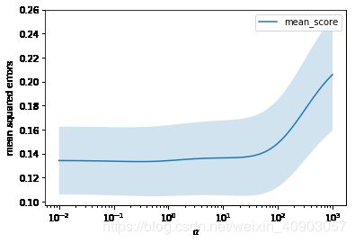(img-KBgDxHs6-1562725477557)(output_66_0.png)]

rcv.coef_

array([ 0.03321449, -0.30956185,  0.05551208,  0.59067449])

手动选择正则化系数——根据业务判断

岭迹图

from sklearn.linear_model import Ridge

ridge = Ridge()

coefs = []
for alpha in alphas:
    ridge.set_params(alpha=alpha)
    ridge.fit(X, y)
    coefs.append(ridge.coef_)

ax = plt.gca()

ax.plot(alphas, coefs)
ax.set_xscale('log')
plt.xlabel('alpha')
plt.ylabel('weights')
plt.title('Ridge coefficients as a function of the regularization')
plt.axis('tight')
plt.show()

[外链图片转存(img-SOMLQtO1-1562725477557)(output_71_0.png)]

ridge.set_params(alpha=0.29)
ridge.fit(X, y)
ridge.coef_

array([ 0.03322236, -0.31025822,  0.05550095,  0.59137388])

ridge.score(X, y)

0.45063153541700307

预测

np.exp(ridge.predict(X_new)[:5])

array([934.79025945, 727.11042209, 703.88143602, 759.04342764,
       709.54172995])

lasso

from sklearn.linear_model import LassoCV

lasso_alphas = np.logspace(-3, 0, 100, base=10)
lcv = LassoCV(alphas=lasso_alphas, cv=10) # Search the min MSE by CV
lcv.fit(X, y)

print('The best alpha is {}'.format(lcv.alpha_))
print('The r-square is {}'.format(lcv.score(X, y))) 
# Default score is rsquared

The best alpha is 0.04037017258596556
The r-square is 0.4426451069862233

from sklearn.linear_model import Lasso

lasso = Lasso()
lasso_coefs = []
for alpha in lasso_alphas:
    lasso.set_params(alpha=alpha)
    lasso.fit(X, y)
    lasso_coefs.append(lasso.coef_)

ax = plt.gca()

ax.plot(lasso_alphas, lasso_coefs)
ax.set_xscale('log')
plt.xlabel('alpha')
plt.ylabel('weights')
plt.title('Lasso coefficients as a function of the regularization')
plt.axis('tight')
plt.show()

[外链图片转存(img-rdcRKGfS-1562725477558)(output_79_0.png)]

lcv.coef_

array([0.        , 0.        , 0.02789489, 0.26549855])

弹性网络

from sklearn.linear_model import ElasticNetCV

l1_ratio = [0.01, .1, .5, .7, .9, .95, .99, 1]

encv = ElasticNetCV(l1_ratio=l1_ratio)
encv.fit(X, y)

ElasticNetCV(alphas=None, copy_X=True, cv=None, eps=0.001, fit_intercept=True,
       l1_ratio=[0.01, 0.1, 0.5, 0.7, 0.9, 0.95, 0.99, 1], max_iter=1000,
       n_alphas=100, n_jobs=1, normalize=False, positive=False,
       precompute='auto', random_state=None, selection='cyclic',
       tol=0.0001, verbose=0)

print('The best l1_ratio is {}'.format(encv.l1_ratio_))
print('The best alpha is {}'.format(encv.alpha_))

The best l1_ratio is 0.01
The best alpha is 1.0998728529638144